6 Conditional Probability

The chances of crashing your car are pretty low, but they’re considerably higher if you’re drunk. Probabilities change depending on the conditions.

We symbolize this idea by writing $\p(A \given B)$, the probability that $A$ is true given that $B$ is true. For example, to say the probability of $A$ given $B$ is 30%, we write: \[ \p(A \given B) = .3. \] We call this kind of probability conditional probability. But how do we calculate conditional probabilities?

6.1 Calculating Conditional Probability

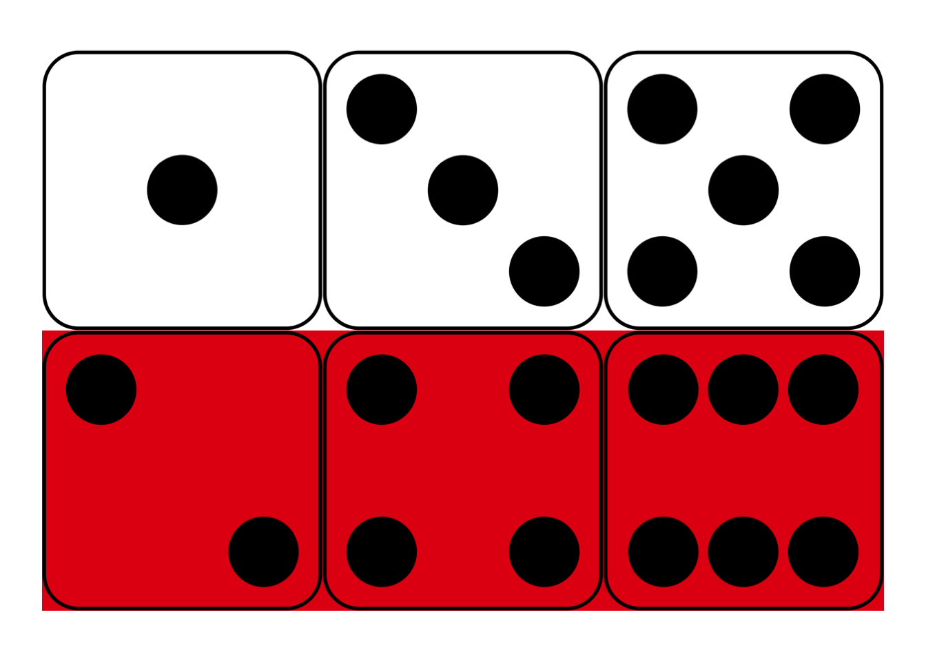
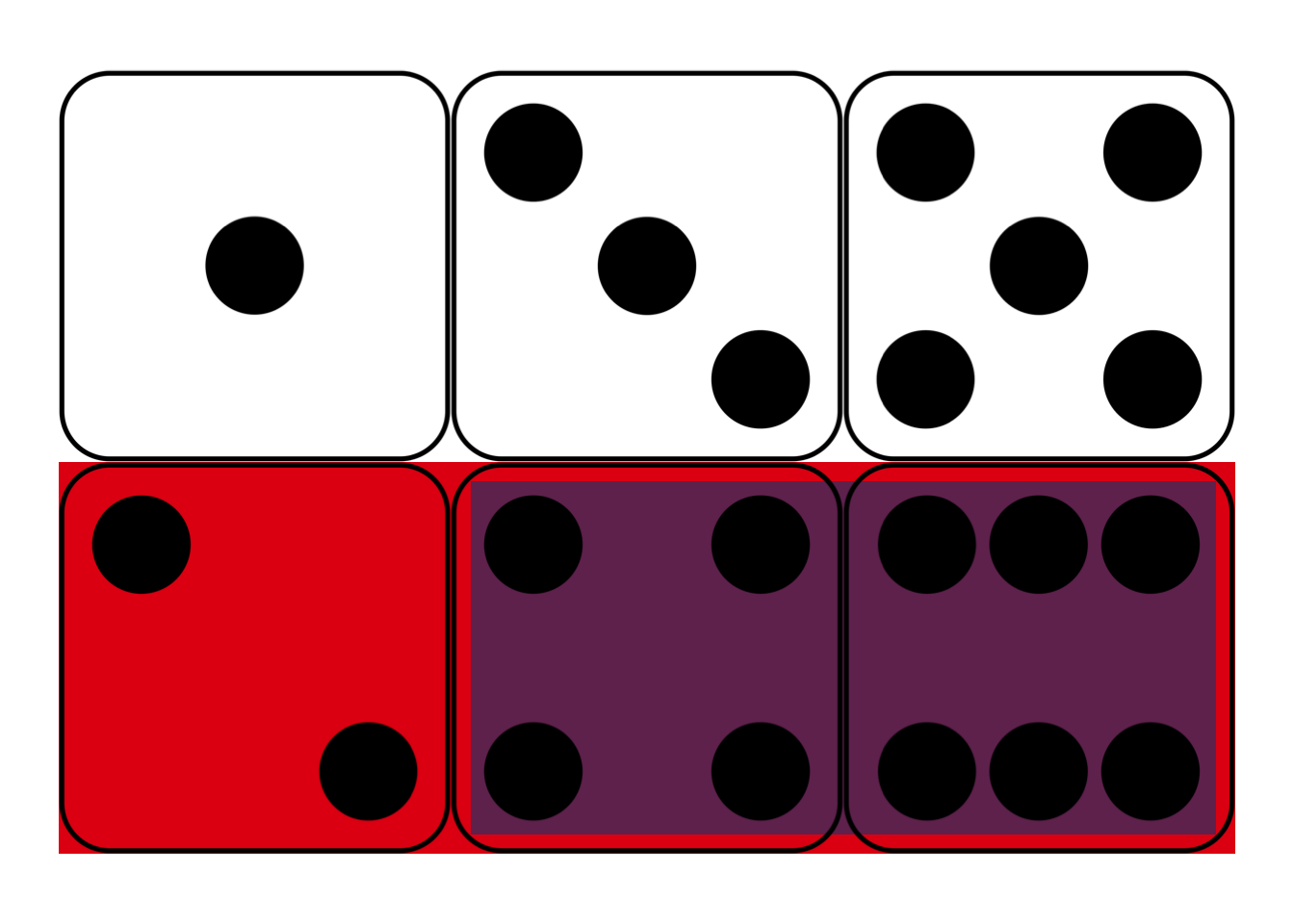Figure 6.1: Conditional probability in a fair die roll

Suppose I roll a fair, six-sided die behind a screen. You can’t see the result, but I tell you it’s an even number. What’s the probability it’s also a “high” number: either a $4$, $5$, or $6$?

Maybe you figured the correct answer: $2/3$. But why is that correct? Because, out of the three even numbers ($2$, $4$, and $6$), two of them are high ($4$ and $6$). And since the die is fair, we expect it to land on a high number $2/3$ of the times it lands on an even number.

This hints at a formula for $\p(A \given B)$.

Conditional Probability: \[ \p(A \given B) = \frac{\p(A \wedge B)}{\p(B)}. \]

In the die-roll example, we considered how many of the $B$ possibilities were also $A$ possibilities. Which means we divided $\p(A \wedge B)$ by $\p(B)$.

In fact, this formula is our official definition for the concept of conditional probability. When we write the sequence of symbols $\p(A \given B)$, it’s really just shorthand for the fraction $\p(A \wedge B) / \p(B)$.

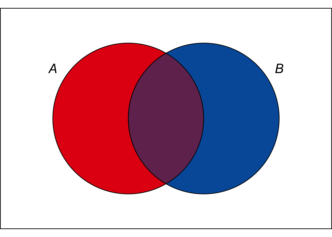$Conditional probability is the size of the $A \wedge B$ region compared to the entire $B$ region.$ Figure 6.2: Conditional probability is the size of the $A \wedge B$ region compared to the entire $B$ region.

In terms of an Euler diagram (Figure 6.2), the definition of conditional probability compares the size of the purple $A \wedge B$ region to the size of the whole $B$ region, purple and blue together. If you don’t mind getting a little colourful with your algebra: \[ \p(A \given B) = \frac{\color{bookpurple}{\blacksquare}}{\color{bookpurple}{\blacksquare} + \color{bookblue}{\blacksquare}}. \] So the definition works because, informally speaking, $\p(A \wedge B)/\p(B)$ is the proportion of the $B$ outcomes that are also $A$ outcomes.

Dividing by zero is a common pitfall with conditional probability. Notice how the definition of $\p(A \given B)$ depends on $\p(B)$ being larger than zero. If $\p(B) = 0$, then the formula ⊕The comedian Steven Wright once quipped that “black holes are where God divided by zero.” \[ \p(A \given B) = \frac{\p(A \wedge B)}{\p(B)} \] doesn’t even make any sense. There is no number that results from the division on the right hand side.33 There are alternative mathematical systems of probability, where conditional probability is defined differently to avoid this problem. But in this book we’ll stick to the standard system. In this system, there’s just no such thing as “the probability of $A$ given $B$” when $B$ has zero probability.

In such cases we say that $\p(A \given B)$ is undefined. It’s not zero, or some special number. It just isn’t a number.

6.2 Conditional Probability & Trees

We already encountered conditional probabilities informally, when we used a tree diagram to solve the Monty Hall problem.

In a tree diagram, each branch represents a possible outcome. The number placed on that branch represents the chance of that outcome occurring. But that number is based on the assumption that all branches leading up to it occur. So the probability on that branch is conditional on all previous branches.

For example, suppose there are two urns of coloured marbles.

Urn X contains 3 black marbles, 1 white.
Urn Y contains 1 black marble, 3 white.

I flip a fair coin to decide which urn to draw from, heads for Urn X and tails for Urn Y. Then I draw one marble at random.

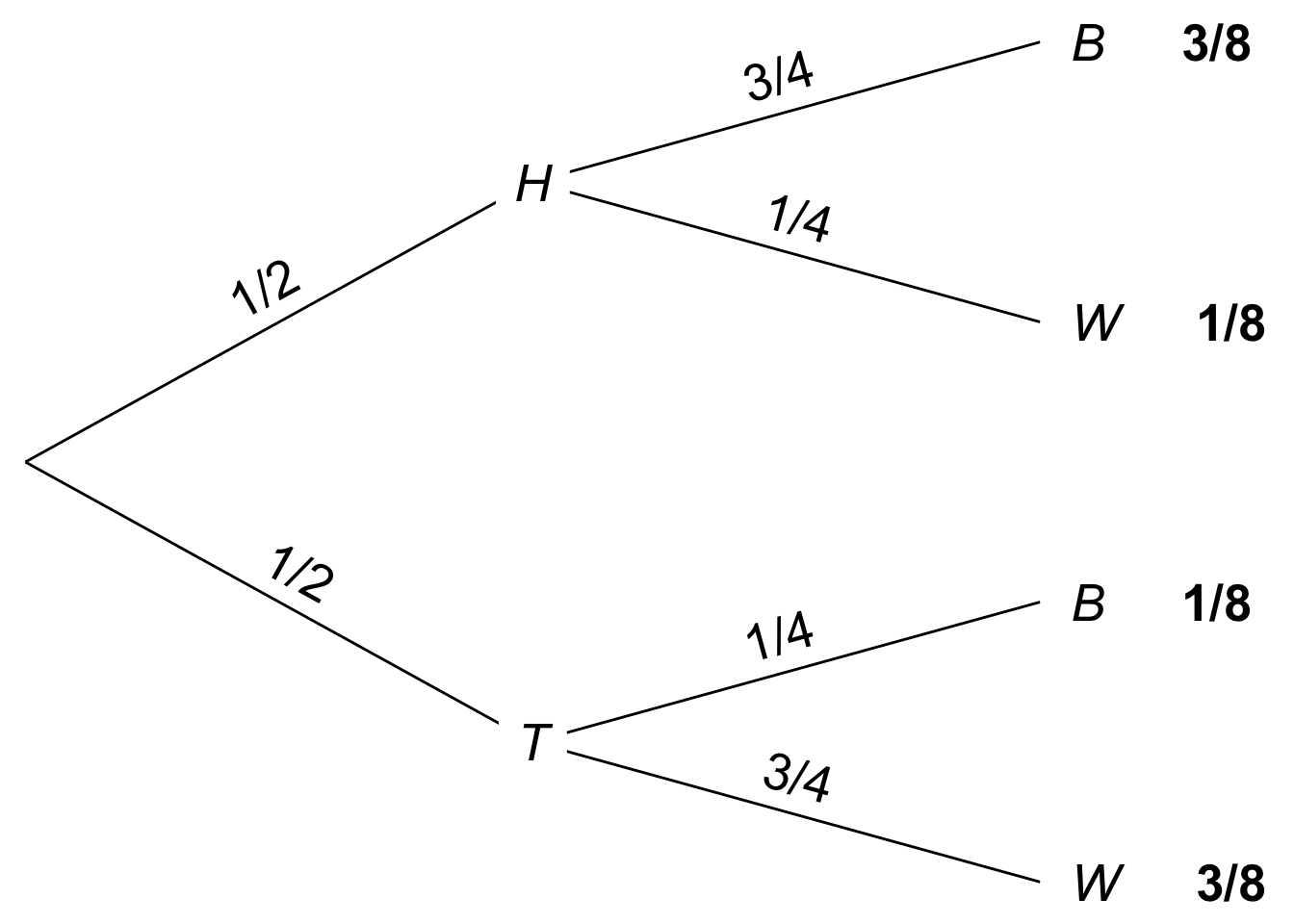Figure 6.3: Tree diagram for an urn problem

In Figure 6.3, the probability of drawing a black marble on the top path is $3/4$ because we are assuming the coin landed heads, and thus I’m drawing from Urn X. If the coin lands tails instead, and I draw from Urn Y, then the chance of a black marble is instead $1/4$. So these quantities are conditional probabilities: \[ \begin{aligned} \p(B \given H) &= 3/4,\\ \p(B \given T) &= 1/4. \end{aligned} \]

Notice, though, the first branch in a tree diagram is different. In the $H$-vs.-$T$ branch, the probabilities are unconditional, since there are no previous branches for them to be conditional on.

6.3 More Examples

Imagine an urn contains marbles of three different colours: 20 are red, 30 are blue, and 40 are green. I draw a marble at random. What is $\p(R \given \neg B)$, the probability it’s red given that it’s not blue? \[ \begin{aligned} \p(R \given \neg B) &= \frac{\p(R \wedge \neg B)}{\p(\neg B)}\\ &= \frac{\p(R)}{\p(\neg B)}\\ &= \frac{20/90}{60/90}\\ &= 1/3. \end{aligned} \] This calculation relies on the fact that $R \wedge \neg B$ is logically equivalent to $R$. A red marble is automatically not blue, so $R$ is true under exactly the same circumstances as $R \wedge \neg B$. The Equivalence Rule thus tells us $\p(R \wedge \neg B) = \p(R)$.

Suppose a university has 10,000 students. Each is studying under one of four broad headings: Humanities, Social Sciences, STEM, or Professional. Under each of these categories, the number of students with an average grade of A, B, C, or D is listed in the following table. What is the probability a randomly selected student will have an A average, given that they are studying either Humanities or Social Sciences?

	Humanities	Social Sciences	STEM	Professional
A	200	600	400	900
B	500	800	1600	900
C	250	400	1500	750
D	50	200	500	450

\[ \begin{aligned} \p(A \given H \vee S) &= \frac{\p(A \wedge (H \vee S))}{\p(H \vee S)}\\ &= \frac{800/10,000}{3,000/10,000}\\ &= 4/15. \end{aligned} \] What about the reverse probability, that a student is studying either Humanities or Social Sciences given that they have an A average? \[ \begin{aligned} \p(H \vee S \given A) &= \frac{\p((H \vee S) \wedge A)}{\p(A)}\\ &= \frac{800/10,000}{2,100/10,000}\\ &= 8/21. \end{aligned} \] Notice how we get a different number now.

6.4 Order Matters

In general, the probability of $A$ given $B$ will be different from the probability of $B$ given $A$. These are different concepts.

For example, university students are usually young, but young people aren’t usually university students. Most aren’t even old enough to be in university. So the probability someone is young given they are in university is high. But the probability someone is in university given that they are young is low. So $\p(Y \given U) \neq \p(U \given Y)$.

Once in a while we do find cases where $\p(A \given B) = \p(B \given A)$. For example, suppose we throw a dart at random at a circular board, divided into four quadrants. The chance the dart will land on the left half given that it lands on the top half is the same as the chance it lands on the top half given it lands on the left. Both probabilities are $1/2$.

But this kind of thing is the exception rather than the rule. Usually, $\p(A \given B)$ will be a different number from $\p(B \given A)$. So it’s important to remember how order matters.

When we write $\p(A \given B)$, we are discussing the probability of $A$. But we are discussing it under the assumption that $B$ is true.

6.5 Declaring Independence

We explained independence informally back in Chapter 4: $A$ and $B$ are independent if the truth of one doesn’t change the probability of the other. Now that we’ve formally defined conditional probability, we can formally define independence too.

Independence: $A$ is independent of $B$ if $\p(A \given B) = \p(A)$ and $\p(A) > 0$.

In other words, they’re independent if $A$’s probability is the same after $B$ is given as it was before (and not just for the silly reason that there was no chance of $A$ being true to begin with).

Now we can establish three useful facts about independence.

The first is summed up in the mantra “independence means multiply.” This actually has two parts.

We already learned the first part with the Multiplication Rule: if $A$ is independent of $B$, then $\p(A \wedge B) = \p(A)\p(B)$. Except now we can see why this rule holds, using the definition of conditional probability and some algebra: \[ \begin{aligned} \p(A \given B) &= \frac{\p(A \wedge B)}{\p(B)} & \mbox{by definition}\\ \p(A \given B)\p(B) &= \p(A \wedge B) & \mbox{by algebra}\\ \p(A)\p(B) &= \p(A \wedge B) & \mbox{by independence}. \end{aligned} \]

The second part of the “independence means multiply” mantra is new though. It basically says that the reverse also holds. As long as $\p(A) > 0$ and $\p(B) > 0$, if $\p(A \wedge B) = \p(A)\p(B)$, then $A$ is independent of $B$.

Bottom line: as long as there are no zeros to worry about, independence is the same thing as $\p(A \wedge B) = \p(A)\p(B)$.

Second, independence is symmetric. If $A$ is independent of $B$, then $B$ is independent of $A$. Informally speaking, if $B$ makes no difference to $A$’s probability, then $A$ makes no difference to $B$’s probability.

This is why we often say “$A$ and $B$ are independent,” without specifying which is independent of which. Since independence goes both ways, they’re automatically independent of each other.

Third, independence extends to negations. If $A$ is independent of $B$, then it’s also independent of $\neg B$ (as long as $\p(\neg B) > 0$, so that $\p(A \given \neg B)$ is well-defined).

Notice, this also means that if $A$ is independent of $B$, then $\neg A$ is independent of $\neg B$ (as long as $\p(\neg A) > 0$).

So far our definition of independence only applies to two propositions. We can extend it to three as follows.

Three-way Independence

$A$, $B$, and $C$ are independent if

$A$ is independent of $B$, $A$ is independent of $C$, and $B$ is independent of $C$, and
$\p(A \wedge B \wedge C) = \p(A)\p(B)\p(C)$.

In other words, a trio of propositions is independent if each pair of them is independent, and the multiplication rule applies to their conjunction. The same idea can be extended to define independence for four propositions, five, etc.

You may be wondering: is part (ii) of this definition really necessary? If each pair of propositions is independent, then the multiplication rule applies to any two of them. Doesn’t this guarantee that it applies to all three together?

Curiously, the answer is no. Suppose someone has equal chances of having been born in the spring, summer, fall, or winter. Let $A$ say that they were born in either spring or summer; let $B$ say they were born in either summer or fall; and let $C$ say they were born in either fall or spring. Pairwise these propositions are all independent. But $\p(A \wedge B \wedge C) = 0$ by the Contradiction rule, since there is no season shared by all three propositions; they cannot all be true. And yet $\p(A)\p(B)\p(C) = 1/8$.

Exercises

Answer each of the following:
1. On a fair die with six sides, what is the probability of rolling a low number (1, 2, or 3) given that you roll an even number.
2. On a fair die with eight sides, what is the probability of rolling an even number given that you roll a high number (5, 6, 7, or 8)?
Suppose $\p(B) = 4/10$, $\p(A) = 7/10$, and $\p(B \wedge A) = 2/10$. What are each of the following probabilities?
1. $\p(A \given B)$
2. $\p(B \given A)$
Five percent of tablets made by the company Ixian have factory defects. Ten percent of the tablets made by their competitor company Guild do. A computer store buys $40\%$ of its tablets from Ixian, and $60\%$ from Guild.

⊕This exercise and the next one are based on very similar exercises from Ian Hacking’s wonderful book, An Introduction to Probability and Inductive Logic.

Draw a probability tree to answer the following questions.
1. What is the probability a randomly selected tablet in the store is made by Ixian and has a factory defect?
2. What is the probability a randomly selected tablet in the store has a factory defect?
3. What is the probability a tablet from this store is made by Ixian, given that it has a factory defect?
In the city of Elizabeth, the neighbourhood of Southside has lots of chemical plants. $2\%$ of Elizabeth’s children live in Southside, and $14\%$ of those children have been exposed to toxic levels of lead. Elsewhere in the city, only $1\%$ of the children have toxic levels of exposure.

Draw a probability tree to answer the following questions.
1. What is the probability that a randomly chosen child from Elizabeth lives in Southside and has toxic levels of lead exposure?
2. What is the probability that a randomly chosen child from Elizabeth has toxic levels of lead exposure?
3. What is the probability that a randomly chosen child from Elizabeth who has toxic levels of lead exposure lives in Southside?
Imagine 100 prisoners are sentenced to death. 70 of them are housed in cell block A, the other 30 are in cell block B. Of the prisoners in cell block A, 9 are innocent. Only 1 prisoner in cell block B is innocent.

The law requires that one prisoner be pardoned. The lucky prisoner will be selected by flipping a fair coin to choose either cell block A or B. Then a fair lottery will be used to select a random prisoner from the chosen cell block.

What is the probability the pardoned prisoner comes from cell block A if she is innocent? Answer each of the following to find out.

$I$ = The pardoned prisoner is innocent.
$A$ = The pardoned prisoner comes from cell block A.
1. What is $Pr(I \given A)$?
2. What is $Pr(A \wedge I)$?
3. What is $Pr(I \given B)$?
4. What is $Pr(B \wedge I)$?
5. What is $Pr(I)$?
6. What is $Pr(A \given I)$?
7. Draw a probability tree to visualize and verify your calculations.
Suppose $A$, $B$, and $C$ are independent, and they each have the same probability: $1/3$. What is $\p(A \wedge B \given C)$?
If $A$ and $B$ are mutually exclusive, what is $\p(A \given B)$? Justify your answer using the definition of conditional probability.
Which of the following situations is impossible? Justify your answer.
1. $\p(A) = 1/2, \p(A \given B) = 1/2, \p(B \given A) = 1/2$.
2. $\p(A) = 1/2, \p(A \given B) = 1, \p(A \given \neg B) = 1$.
Is the following statement true or false: if $A$ and $B$ are mutually exclusive, then $Pr(A \vee B \given C) = Pr(A \given C) + Pr(B \given C)$. Justify your answer.
Justify the second part of the “independence means multiply” mantra: if $\p(A) > 0$, $\p(B) > 0$, and $\p(A \wedge B) = \p(A) \p(B)$, then $A$ is independent of $B$.

Hint: start by supposing $\p(A) > 0$, $\p(B) > 0$, and $\p(A \wedge B) = \p(A)\p(B)$. Then apply some algebra and the definition of conditional probability.
Justify the claim that independence is symmetric: if $A$ is independent of $B$, then $B$ is independent of $A$.

Hint: start by supposing that $A$ is independent of $B$. Then write out $\p(A \given B)$ and apply the definition of conditional probability.
Suppose $A$, $B$, and $C$ are independent. Is it possible that $\p(A \wedge B \wedge C) = 0$? If yes, give an example where this happens. If no, prove that it cannot happen.
Suppose we have $4$ apples and $10$ buckets. We place each apple in a random bucket; the placement of each apple is independent of the others. Let $B_{ij}$ be the proposition that apples $i$ and $j$ were placed in the same bucket.
1. Is $B_{12}$ independent of $B_{34}$?
2. Is $B_{12}$ independent of $B_{23}$?
3. Is every pair of $B_{ij}$ propositions independent?
4. Is every trio of $B_{ij}$ propositions independent?
Suppose we have a coin whose bias we want to learn, so we’re going to flip it $3$ times. We start out by assigning the same probability to each possible sequence of heads and tails. For example, the sequences $HTH$ and $TTT$ are equally likely, as are all other sequences.
1. Before we do our $3$ flips, what is the probability of $HTH$?
2. What is the probability of heads on the third flip, given that the first two flips land heads?
Prove that if $A$ logically entails $B$, then $\p(B \given A) = 1$.
Suppose the following three conditions hold:
1. $\p(A) = \p(\neg A)$,
2. $\p(B \given A) = \p(B \given \neg A)$,
3. $\p(B) > 0$.
Must the following be true then?
1. $\p(A \given B) = \p(A \given \neg B) = 1/2$?
If yes, prove that (iv) must hold. If no, give a counterexample: draw an Euler diagram where conditions (i)–(iii) hold, but not (iv).
Prove that the equation $\p(A \given B) \p(B) = \p(B \given A) \p(A)$ always holds. (Assume both conditional probabilities are well-defined.)
Prove that the following equation always holds, assuming the conditional probabilities are well-defined: \[ \frac{\p(A \given B)}{\p(B \given A)} = \frac{\p(A)}{\p(B)}. \]
Does the equation $\p(A \given B) = \p(\neg B \given \neg A)$ always hold, assuming both conditional probabilities are both well-defined? If yes, prove that it does. If no, draw an eikosogram where it fails to hold.
Suppose an urn contains 30 black marbles and 70 white. We randomly draw 5 marbles with replacement. Let $A$ be the proposition that $3$ of the first $4$ draws are black, and let $B$ be the proposition that the $5$^th draw is black. Calculate the following quantity: \[ \frac{Pr(A \,\vert\, B)}{Pr(B \,\vert\, A)} \frac{Pr(B)}{Pr(A)}. \]