7 Calculating Probabilities, Part 2

We learned rules for $\vee$ and $\wedge$ back in Chapter 5.

The Addition Rule: $\p(A \vee B) = \p(A) + \p(B)$ if $A$ and $B$ are mutually exclusive.
The Multiplication Rule: $\p(A \& B) = \p(A) \times \p(B)$ if $A$ and $B$ are independent.

In this chapter we’ll learn new, more powerful rules for $\vee$ and $\wedge$. But we’ll start with negation, a rule for calculating $\p(\neg A)$.

7.1 The Negation Rule

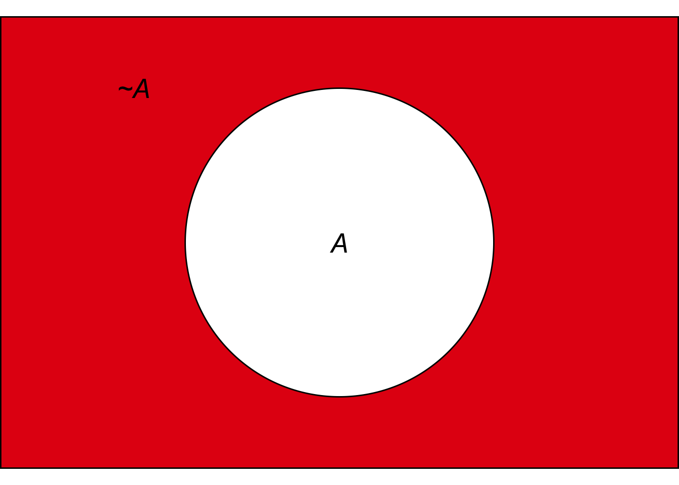$The Negation Rule. $\p(\neg A) = 1 - \p(A)$.$ Figure 7.1: The Negation Rule. $\p(\neg A) = 1 - \p(A)$.

If there’s a 70% chance of rain, then there’s a 30% chance it won’t rain. In symbols, if $\p(R) = .7$ then $\p(\neg R) = .3$. So the rule for $\p(\neg A)$ is:

The Negation Rule: $\p(\neg A) = 1 - \p(A)$.

In terms of an Euler diagram, the probability of $\neg A$ is the size of the red region. So $\p(\neg A)$ is $1 - \p(A)$.

Notice that this rule can be flipped around, to calculate the probability of a positive statement: \[ \p(A) = 1 - \p(\neg A). \] Sometimes what we want to know is $\p(A)$, but it turns out to be much easier to calculate $\p(\neg A)$ first. Then we use this flipped version of the negation rule to get what we’re after.

7.2 The General Addition Rule

The Addition Rule for calculating $\p(A \vee B)$ depends on $A$ and $B$ being mutually exclusive. What if they’re not? Then we can use:

The General Addition Rule: $\p(A \vee B) = \p(A) + \p(B) - \p(A \wedge B)$.

This rule always applies, whether $A$ and $B$ are mutually exclusive or not.

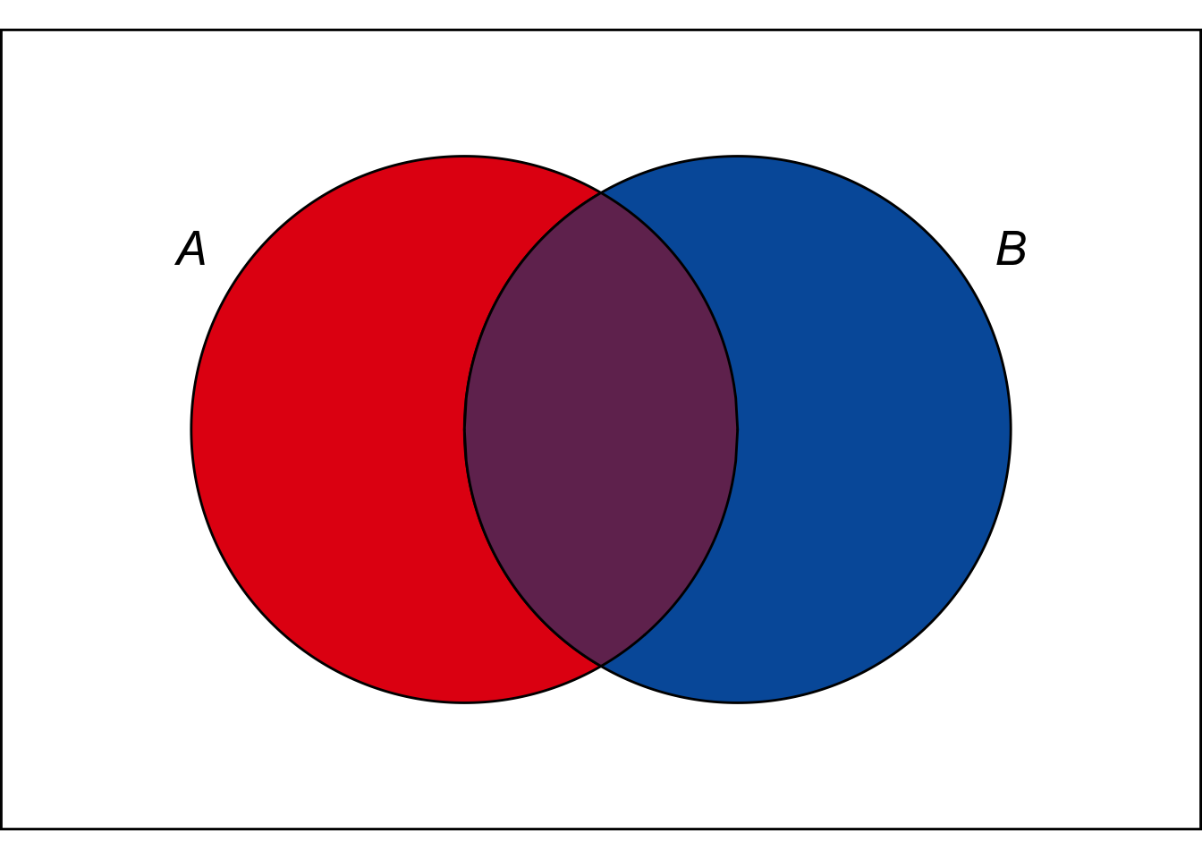Figure 7.2: The General Addition Rule in an Euler diagram.

To understand the rule, consider an Euler diagram where $A$ and $B$ are not mutually exclusive. In terms of colour, the size of the $A \vee B$-region is: \[ \color{bookred}{\blacksquare}\color{black}{} \,+\, \color{bookpurple}{\blacksquare}\color{black}{} \,+\, \color{bookblue}{\blacksquare}\color{black}{}. \] Which is the same as: \[ (\color{bookred}{\blacksquare}\color{black}{} \,+\, \color{bookpurple}{\blacksquare}\color{black}{}) \,+\, (\color{bookblue}{\blacksquare}\color{black}{} \,+\, \color{bookpurple}{\blacksquare}\color{black}{}) \,-\, \color{bookpurple}{\blacksquare}\color{black}{}. \] In algebraic terms this is: \[ \p(A) + \p(B) - \p(A \wedge B).\]

To think of it another way, when we add $\p(A) + \p(B)$ to get the size of the $A \vee B$ region, we double-count the $A \wedge B$ region. So we have to subtract out $\p(A \wedge B)$ at the end.

What if there is no $A \wedge B$ region? Then $\p(A \wedge B) = 0$, so subtracting it at the end has no effect. Then we just have the old Addition Rule: \[ \begin{aligned} \p(A \vee B) &= \p(A) + \p(B) - \p(A \wedge B)\\ &= \p(A) + \p(B) - 0\\ &= \p(A) + \p(B).\\ \end{aligned} \] And this makes sense. If there is no $A \wedge B$ region, that means $A$ and $B$ are mutually exclusive. So the old Addition Rule applies.

That’s why we call the new rule the General Addition Rule. It applies in general, even when $A$ and $B$ are not mutually exclusive. And in the special case where they are mutually exclusive, it gives the same result as the Addition Rule we already learned.

A tree diagram also works to explain the General Addition Rule. Consider Figure 7.3, where we start with branches for $A$ and $\neg A$, then subdivide into branches for $B$ and $\neg B$.

Figure 7.3: Tree diagram with the three $A \vee B$ leaves marked

$Tree diagram with the three $A \vee B$ leaves marked$

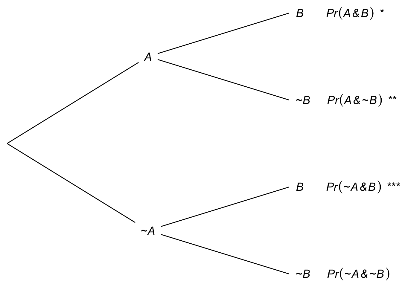
There are three leaves where $A \vee B$ is true, marked with asterisks. If we add $\p(A) + \p(B)$, we’re adding the two leaves where $A$ is true (* and **) to the two leaves where $B$ is true (* and ***). So we’ve double-counted the $A \wedge B$ leaf (*). To get $\p(A \vee B)$ then, we have to subtract one of those $A \wedge B$ leaves (*).

There is a catch to the General Addition Rule. You need to know $\p(A \wedge B)$ in order to apply it. Sometimes that information is given to us. But when it’s not, we have to figure it out somehow. If $A$ and $B$ are mutually exclusive, then it’s easy: $\p(A \wedge B) = 0$. Or, if they’re independent, then we can calculate $\p(A \wedge B) = \p(A) \times \p(B)$. But in other cases we have to turn elsewhere.

7.3 The General Multiplication Rule

How can we calculate $\p(A \wedge B)$ in general?

The General Multiplication Rule: $\p(A \wedge B) = \p(A \given B) \p(B).$

The intuitive idea is, if you want to know how likely it is $A$ and $B$ will both turn out to be true, first ask yourself how likely $A$ is to be true if $B$ is true. Then weight the answer according to $B$’s chances of being true.

Notice, if $A$ and $B$ are independent, then this rule just collapses into the familiar Multiplication Rule we already learned. If they’re independent, then $\p(A \given B) = \p(A)$ by definition. So substituting into the General Multiplication Rule gives: \[ \begin{aligned} \p(A \wedge B) &= \p(A \given B) \p(B)\\ &= \p(A) \p(B). \end{aligned} \] Which is precisely the Multiplication Rule.

So we now have two rules for $\wedge$. The first one only applies when the two sides of the $\wedge$ are independent. The second applies whether they’re independent or not. The second rule ends up being the same as the first one when they are independent.

A tree diagram helps us understand this rule too. Recall this problem from Chapter 6, with two urns of coloured marbles:

Urn X contains 3 black marbles, 1 white.
Urn Y contains 1 black marble, 3 white.

I flip a fair coin to decide which urn to draw from, heads for Urn X and tails for Urn Y. Then I draw one marble at random.

Figure 7.4: Tree diagram for an urn problem

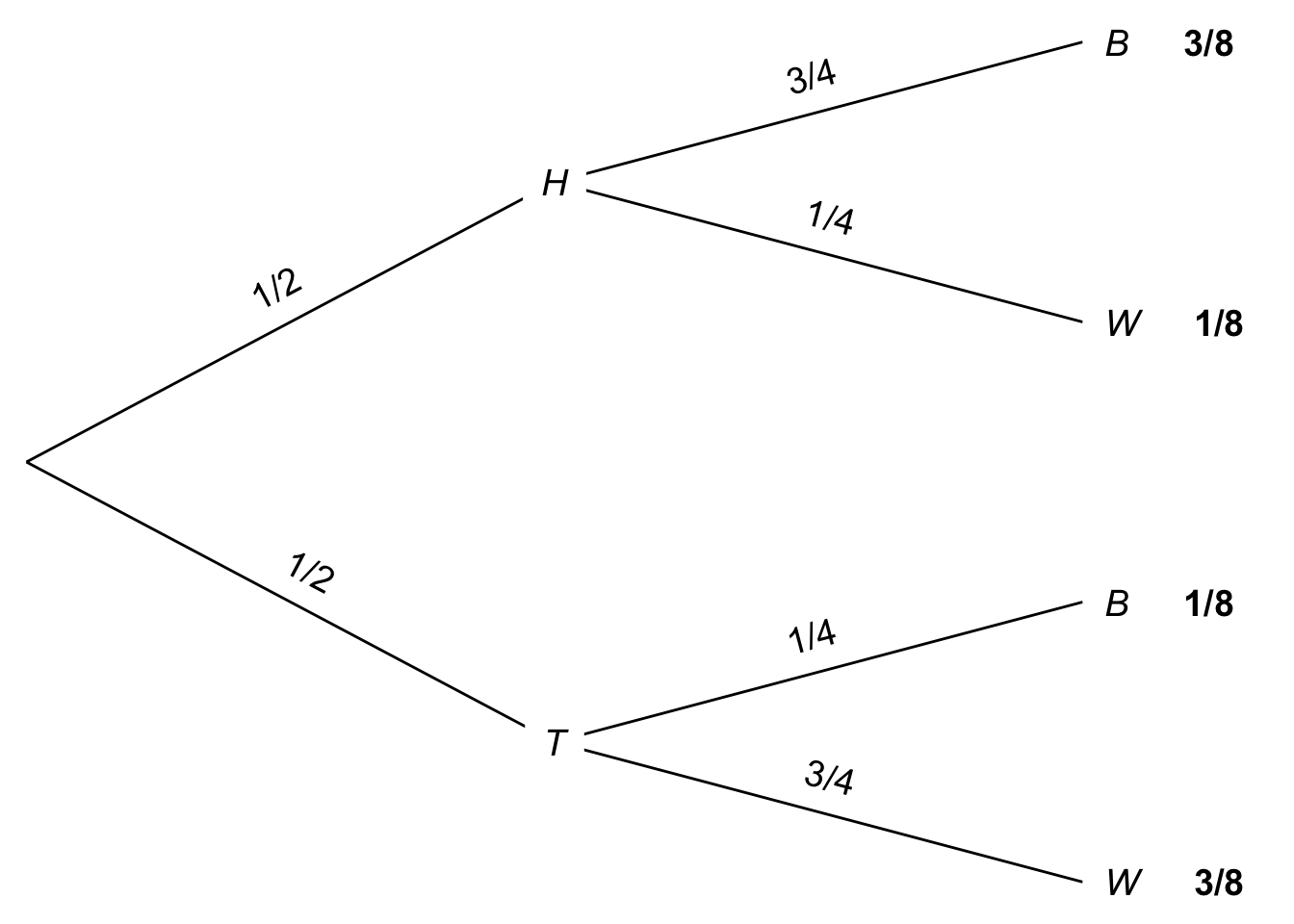
Now suppose we want to know the probability the coin will land tails and the marble drawn will be white, $\p(T \wedge W)$. The General Multiplication Rule tells us the answer is: \[ \begin{aligned} \p(T \wedge W) &= \p(W \wedge T)\\ &= \p(W \given T) \p(T)\\ &= 3/4 \times 1/2\\ &= 3/8. \end{aligned} \] In the tree diagram, this corresponds to following the bottom-most path, multiplying the probabilities as we go. And this makes sense: half the time the coin will land tails, and on $3/4$ of those occasions the marble drawn will be white. So, if we were to repeat the experiment again and again, we would get tails followed by a white marble in $3$ out of every $8$ trials.

Black hole warning: notice that the General Multiplication Rule depends on $\p(A \given B)$ being well-defined. So it only applies when $\p(B) \gt 0$.

7.4 Laplace’s Urn Puzzle

The same urn scenario was used by 18th Century mathematician Laplace in one of his favourite puzzles. He asked what happens if we do two draws, with replacement. What’s the probability both draws will come up black?

It’s tempting to say $1/4$. The probability of drawing a black marble on each draw is $1/2$. So it seems the probability of two blacks is just $1/2 \times 1/2 = 1/4$.

But the correct answer is actually $5/16$. Why? Let’s use a probability tree again.

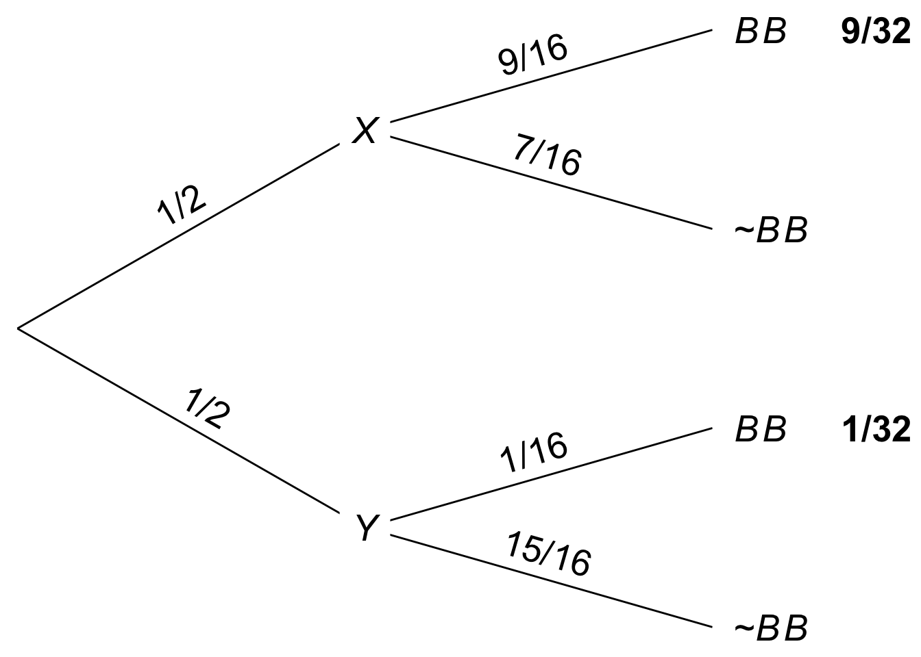Figure 7.5: Building a probability tree to solve Laplace’s urn puzzle

Depending on how the coin lands, you could end up drawing either from Urn X or from Urn Y, with equal probability.

If you end up drawing from Urn X, the probability of a black marble on any given draw is $3/4$. We’re drawing with replacement, so this doesn’t change on the second draw. The probability both draws will come up black is thus $3/4 \times 3/4 = 9/16$.

If instead you end up drawing from Urn Y, the probability of a black marble on any given draw is $1/4$. And this doesn’t change on the second draw since we’re drawing with replacement. So the chance of both being black in this case is $1/4 \times 1/4 = 1/16$.

So the probability of drawing two black marbles from Urn X is: \[ \begin{aligned} \p(X \wedge BB) &= \p(X) \p(BB \given X)\\ &= 1/2 \times 9/16\\ &= 9/32. \end{aligned} \] And the probability of drawing two black marbles from Urn Y is: \[ \begin{aligned} \p(Y \wedge BB) &= \p(Y) \p(BB \given Y)\\ &= 1/2 \times 1/16\\ &= 1/32. \end{aligned} \] Now we can apply the Addition Rule to calcualte $\p(BB)$: \[ \begin{aligned} \p(BB) &= \p(X \wedge BB) + \p(Y \wedge BB)\\ &= 9/32 + 1/32\\ &= 5/16. \end{aligned} \]

7.5 The Law of Total Probability

This kind of calculation comes up a lot. Since it would be tedious to figure it out from scratch every time, we make a general rule instead:

The Law of Total Probability: $\p(A) = \p(A \given B) \p(B) + \p(A \given \neg B) \p(\neg B)$.

There’s an intuitive idea at work here. To figure out how likely $A$ is, consider how likely it would be if $B$ were true, and how likely it would be if $B$ were false. Then weight each of those hypothetical possibilities according to their probabilities.

Figure 7.6: The Law of Total Probability calculates the size of the $A$ region by summing its two parts.

We can also use an Euler diagram. The size of the $A$ region is the sum of the $A \wedge B$ region and the $A \wedge \neg B$ region: $\color{bookpurple}{\blacksquare}\color{black}{} + \color{bookred}{\blacksquare}\color{black}{}$. And each of those regions can be calculated using the General Multiplication Rule. For example, $\p(A \wedge B) = \p(A \given B) \p(B)$. So in algebraic terms we have: \[ \begin{aligned} \p(A) &= \color{bookpurple}{\blacksquare}\color{black}{} + \color{bookred}{\blacksquare}\color{black}{}\\ &= \p(A \wedge B) + \p(A \wedge \neg B)\\ &= \p(A \given B) \p(B) + \p(A \given \neg B) \p(\neg B). \end{aligned} \] Which is precisely the Law of Total Probability.

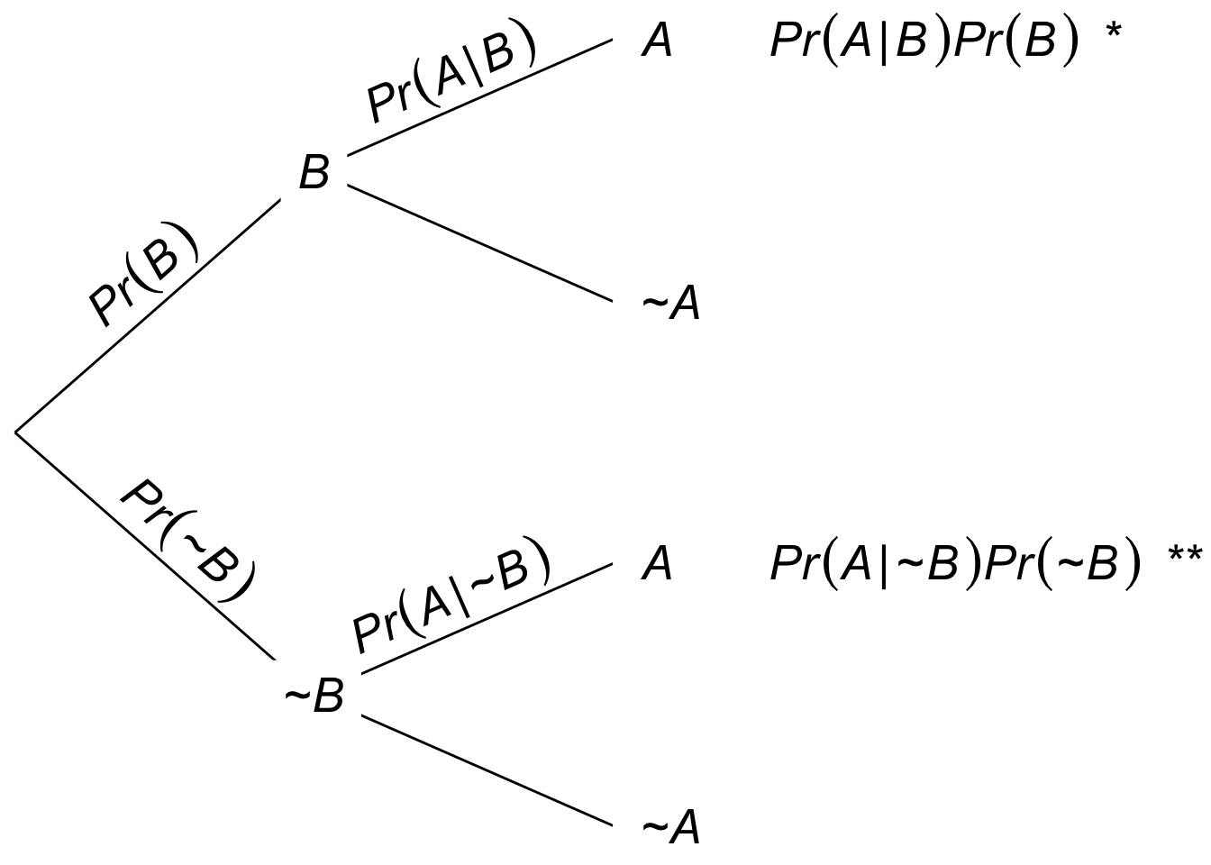Figure 7.7: The Law of Total Probability in a tree diagram

We can also use a tree diagram to illustrate the same reasoning. There are two leaves where $A$ is true, marked with asterisks. To get the probability of each leaf we multiply across the branches (that’s the General Multiplication Rule). And then to get the total probability for $A$, we add up the two leaves: $\p(A) = * + **$. Once again the result is the Law of Total Probability: \[ \p(A) = \p(A \given B) \p(B) + \p(A \given \neg B) \p(\neg B). \]

Black hole warning: notice that the Law of Total Probability depends on $\p(A \given B)$ and $\p(A \given \neg B)$ both being well-defined. So it only applies when $\p(B) \gt 0$ and $\p(\neg B) \gt 0$.

7.6 Example

Every day Professor X either drives her car to campus or takes the bus. Mostly she drives, but one time in four she takes the bus. When she drives, she’s on time $80\%$ of the time. When she takes the bus, she’s on-time $90\%$ of the time. What is the probability she’ll be on time for class tomorrow?

First let’s solve this by just applying the Law of Total Probability directly: \[ \begin{aligned} \p(O) &= \p(O \given B)\p(B) + \p(O \given D)\p(D)\\ &= (9/10)(1/4) + (8/10)(3/4)\\ &= 33/40. \end{aligned} \] Now let’s solve it slightly differently, thinking the problem through from more basic principles.

There are two, mutually exclusive cases where Professor X is on time: one where she takes the bus, one where she drives. \[ \p(O) = \p(O \wedge B) + \p(O \wedge D). \] We can use the General Multiplication Rule to calculate the probability she’ll take the bus and be on time: \[ \p(O \wedge B) = \p(O \given B)\p(B). \] And we can do the same for the probability she’ll drive and be on time: \[ \p(O \wedge D) = \p(O \given D)\p(D)\] Putting all the pieces together: \[ \begin{aligned} \p(O) &= \p(O \wedge B) + \p(O \wedge D)\\ &= \p(O \given B)\p(B) + \p(O \given D)\p(D)\\ &= (9/10)(1/4) + (8/10)(3/4)\\ &= 33/40. \end{aligned} \]

Notice that we didn’t just get the same answer, we ended up doing the same calculation too. Our second approach just reconstructed from scratch the reasoning behind the Law of Total Probability. It’s a very good idea to understand the rationale behind the Law of Total Probability. But once you get used to the formula, it’s also fine to skip straight to applying it directly.

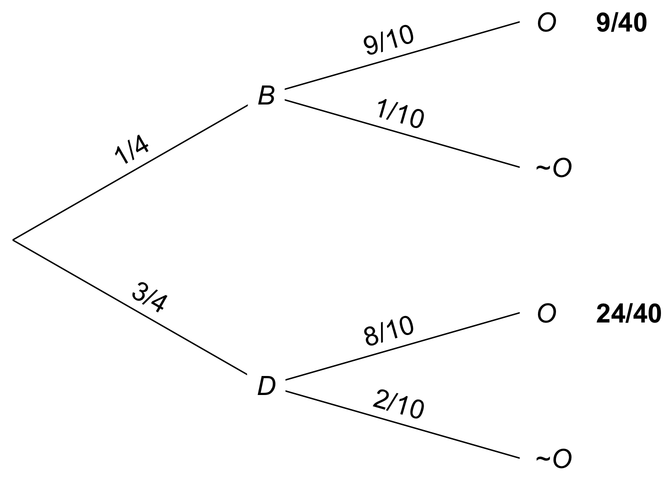Figure 7.8: A probability tree for Professor X

You can also use a tree diagram. Again, the calculation will be the same. But the diagram may help you get started, and it helps you check that you’ve applied the formula correctly too.

Exercises

Suppose you have an ordinary deck of $52$ playing cards, and you draw one card at random. What is the probability you will draw:
1. A face card (king, queen, or jack)?
2. A card that is not a face card?
3. An ace or a spade?
4. A queen or a heart?
5. A queen or a non-spade?
Suppose that $Pr(A)=1/3$, $Pr(B) = 1/4$, and that $A$ and $B$ are independent. What is $\p(\neg A \wedge \neg B)$?
What is $\p(X \vee B)$ in the first version of the urn problem? (The first version is the one where we start with a fair coin flip to choose between Urn X and Urn Y, then draw one marble at random.)
Recall Laplace’s version of the urn puzzle: we select either Urn X or Urn Y at random, then we do two random draws from it, with replacement. What is $\p(X \vee BB)$?
Suppose we add a third urn to Laplace’s puzzle: Urn Z contains $2$ black marbles and $2$ white ones. We choose one of the three urns at random, and then do two random draws with replacement. What is $\p(BB)$ then?
The Law of Total probability calculates $\p(A)$ by considering two cases, $B$ and $\neg B$. Notice that $B$ and $\neg B$ form a partition: they are mutually exclusive and exhaustive possibilities.

Suppose we had a partition of three propositions instead: $B$, $C$, and $D$. Would the following extension of the Law of Total Probability hold then? \[\p(A) = \p(A \given B)\p(B) + \p(A \given C)\p(C) + \p(A \given D)\p(D).\] Justify your answer.
Suppose there are two urns with the following contents:
- Urn I has 8 black balls, 2 white.
- Urn II has 2 black balls, 3 white.
A fair coin will be flipped. If it comes up heads, a ball will be drawn from Urn I at random. Otherwise a ball will be drawn from Urn II at random. What is the probability a black ball will be drawn?
Suppose you have an ordinary deck of 52 cards. A card is drawn and is not replaced, then another card is drawn. Assume that on each draw all the cards then in the deck have an equal chance of being drawn.
1. What is the probability of getting an ace on draw 1?
2. What is the probability of a ten on draw 2 given ace on draw 1?
3. What is the probability of an ace on draw 1 and a ten on draw 2?
4. What is the probability of a ten on draw 1 and an ace on draw 2?
5. What is the probability of an ace and a ten?
6. What is the probability of 2 aces?
The probability that George will study for the final is $4/5$. The probability he will pass given that he studies is $3/5$. The probability he will pass given that he does not study is $1/10$. What is the probability George will pass?
Calculate each of the following probabilities:
1. $Pr(P) = 1/2$, $Pr(Q) = 1/2$, $Pr(P \wedge Q) = 1/8$. What is $Pr(P \vee Q)$?
2. $Pr(R) = 1/2, Pr(S) = 1/4, Pr(R \vee S) = 3/4$. What is $Pr(R \wedge S)$?
3. $Pr(U) = 1/2, Pr(T) = 3/4, Pr(U \wedge \neg T) = 1/8$. What is $Pr(U \vee \neg T)$?
$Pr(P) = 1/2, Pr(Q) = 1/2$, and $P$ and $Q$ are independent.
1. What is $Pr(P {\,\&\,}Q)$?
2. Are $P$ and $Q$ mutually exclusive?
3. What is $Pr(P \vee Q)$?
Suppose $A$, $B$, and $C$ are all mutually exclusive, and they each have the same probability: $1/5$. What is $\p(\neg(A \wedge B) \wedge C)$?
Researchers are studying the safety of drug X. They enroll 60 subjects in a study and give drug X to 35 of them. By the end of the study, 5 subjects have developed stomach cancer: 3 who were taking drug X, 2 who were not.

Draw a Venn diagram and use it to answer the following questions about a randomly selected subject:
1. What is the probability they developed stomach cancer?
2. What is the probability they developed stomach cancer given that they were taking drug X?
3. What is the probability they developed stomach cancer given that they were not taking drug X?
4. Based on this study, would you conclude that drug X increases or decreases the risk of stomach cancer?
There is a room filled with two types of urns.
- Type A urns contain 30 yellow marbles, 70 red.
- Type B urns contain 20 green marbles, 80 yellow.
The two types of urn look identical, but 80% of them are Type A.
1. You pick an urn at random and draw a marble from it at random. What is the probability the marble will be yellow?
2. You look at the marble: it is yellow. What’s the probability the urn is a Type B urn?
Suppose $A$, $B$, and $C$ are independent of one another. Does it follow that $\p(B \given A \wedge C) = \p(B)$? Justify your answer.
Is the following combination of probabilities possible? $Pr(A) = 2/5$, $Pr(B) = 4/5$, and $Pr(A \vee B) = 3/5$. Justify your answer.
Which of the following situations is impossible? Justify your answer.
1. $\p(A) = 4/5$, $\p(B) = 1/5$, $\p(\neg A \wedge B) = 3/5$.
2. $\p(\neg X) = 1/3$, $\p(\neg Y) = 2/3$, $\p(X \wedge Y) = 0$.
If $Pr(A)=0$, what is $\p(A \given B)$? Justify your answer.
If $A$ and $B$ are logically equivalent, what is $\p(A \given B)$? Justify your answer.
Suppose $A$, $B$, and $C$ all have the same probability, namely $1/4$. Suppose they are also independent of one another. What is $\p(\neg A \vee \neg B \vee \neg C)$?

Hint: $\neg A \vee \neg B \vee \neg C$ is logically equivalent to $\neg (A \wedge B \wedge C)$. Why?
If $\p(A) = 1/2$ and $\p(B) = 3/5$, are $A$ and $B$ mutually exclusive? Justify your answer.
Suppose $\p(A) = 1/4$, $\p(B) = 1/3$, and $A$ and $B$ are independent. What is $\p(A \vee (B \wedge \neg A))$?
Suppose $A$ logically entails $C$, and $A$ and $B$ are independent. If $\p(A) = 1/7$, $\p(B) = 1/3$, and $\p(C)=1/3$, what is $\p((A \wedge \neg B) \vee \neg C)$?
If $A$ and $B$ are mutually exclusive, must the following hold? \[\p(A \vee B \given C) = \p(A \given C) + \p(B \given C).\] Assume the conditional probabilities are all well-defined, and justify your answer.

Hint: apply the definition of conditional probability and use the following fact: $(A \vee B) \wedge C$ is logically equivalent to $(A \wedge C) \vee (B \wedge C)$.
Prove that if $A$ and $B$ are mutually exclusive, then \[\p(A \given A \vee B) = \frac{ \p(A) }{ \p(A) + \p(B) }.\]
If $\p(C \given B \wedge A) = \p(C \given B)$, does this follow? \[\p(A \given B \wedge C) = Pr(A \given B).\] Assume all conditional probabilities are well-defined, and justify your answer.
Justify the claim from Chapter 6 that independence extends to negations: if $A$ is independent of $B$, then it’s also independent of $\neg B$ (provided $\p(\neg A) > 0$).

Warning: this one is hard. I suggest starting with the equation: \[ \p(A \wedge B) = \p(A) \p(B). \] Then use the Negation Rule which tells us: \[ \p(B) = 1 - \p(\neg B). \] And use the Addition Rule to get: \[ \p(A \wedge B) = \p(A) - \p(A \wedge \neg B).\]
Three friends get together and tell each other their birthdays. If each person’s birthday is independent of the others, what is the probability that they all have different birthdays? Assume birthdays are randomly distributed, and ignore leap years; each friend has a $1/365$ chance of being born on a given day.
An urn has two marbles, one black and one white. We will do repeated random draws, with replacement. But every time we draw a white marble, another white marble will be added to the urn for the next draw. Suppose we do $5$ draws. What is the probability they will all be white?
Consider the inequality $\p(A) < \p(A \vee B)$. Which of the following is correct?
1. This inequality always holds.
2. This inequality only holds sometimes: when $A$ and $B$ are mutually exclusive.
3. This inequality only holds sometimes: when $A$ and $B$ are compatible (not mutually exclusive).
4. This inequality only holds sometimes: when $\p(\neg A \wedge B) > 0$.
5. This inequality never holds.
Consider the following two statements.
1. If $\p(A \given B) = 2/3$ and $\p(A \given \neg B) = 2/3$, then $\p(A) = 2/3$.
2. If $\p(A) = 2/3$, then $\p(A \given B) = 2/3$ and $\p(A \given \neg B) = 2/3$.
Assuming all conditional probabilities are well-defined, which of these statements is true? Both, neither, or just one (which one)?
Consider the following two assignments of probabilities.
1. $\p(X \wedge Y) = 1/4$, $\p(X \wedge \neg Y) = 1/4$, $\p(\neg X) = 1/2$.
2. $\p(A \wedge \neg B) = 1/3$, $\p(A) = 1/2$, $\p(B) = 1/4$.
Which of them violate the laws of probability: both, neither, or just one (which one)?
Consider the following two assignments of probabilities.
1. $\p(A) = 1/3$, $\p(A \wedge B) = 1/9$, $\p(\neg B \given A) = 2/9$.
2. $\p(X \given Y) = 1/3$, $\p(X \given \neg Y) = 1/2$, $\p(X) = 2/3$.
Which of them violate the laws of probability: both, neither, or just one (which one)?
Consider the following two assignments of probabilities:
1. $\p(A) = 4/5$, $\p(B) = 1/5$, $\p(\neg A \wedge B) = 3/5$.
2. $\p(\neg X) = 1/10$, $\p(\neg Y) = 9/10$, $\p(X \wedge Y) = 0$.
Which of them violate the laws of probability: both, neither, or just one (which one)?
In April of 2021 during the Covid-19 pandemic, concerns arose about the safety of one of the vaccines. At the time $7$ million people had already received this vaccine, a few of whom developed dangerous bloodclots. One of these people had already died as a result. ⊕This exercise is based on a tweet of Nate Silver’s

Suppose at the time there was a $1/100$ chance of getting Covid-19 without the vaccine, and only a $1/1,000$ chance with the vaccine. And suppose unvaccinated people who got Covid-19 died in $1/150$ cases, while those who’d had the vaccine only died in $1/500$ cases.

What then was the probability of dying, either from a vaccine-induced blood clot or from Covid-19, if you did take the vaccine? What was the probability if you didn’t? (Assume no other vaccines were available.)
Prove that if $\p(B) = 1$, then $\p(A \wedge B) = \p(A)$.
Prove that $\p(A \wedge B) \geq \p(A) + \p(B) - 1$.
Prove that $\p(A \wedge B \wedge C) = \p(A) \p(B \given A) \p(C \given B \wedge A)$ as long as the two conditional probabilities are well-defined.