In an earlier post we met the $\lambda$-continuum, a generalization of Laplace’s Rule of Succession. Here is Laplace’s rule, stated in terms of flips of a coin whose bias is unknown.

The Rule of Succession: Given $k$ heads out of $n$ flips, the probability the next flip will land heads is $$\frac{k+1}{n+2}.$$

To generalize we introduce an adjustable parameter, $\lambda$. Intuitively $\lambda$ captures how cautious we are in drawing conclusions from the observed frequency.

The $\lambda$ Continuum: Given $k$ heads out of $n$ flips, the probability the next flip will land heads is $$\frac{k + \lambda / 2}{n + \lambda}.$$

When $\lambda = 2$, this just is the Rule of Succession. When $\lambda = 0$, it becomes the “Straight Rule,” which matches the observed frequency, $k/n$. The general pattern is: the larger $\lambda$, the more flips we need to see before we tend toward the observed frequency, and away from the starting default value of $1/ 2$.$\newcommand{\p}{P}\newcommand{\given}{\mid}\newcommand{\dif}{d}$

So what’s so special about $\lambda = 2$? Why did Laplace and others take a special interest in the Rule of Succession? Because it derives from the Principle of Indifference. We saw that setting $\lambda = 2$ basically amounts to assuming all possible frequencies have equal prior probability. Or that all possible biases of the coin are equally likely. The Rule of Succession thus corresponds to a uniform prior.

What about other values of $\lambda$ then? What kind of prior do they correspond to? This question has an elegant and illuminating answer, which we’ll explore here.

PDF version here

A Preview

Let’s preview the result we’ll arrive at. Because, although the core idea isn’t very technical, deriving the full result does takes some noodling. It will be good to have some sense of where we’re going.

Here’s a picture of the priors that correspond to various choices of $\lambda$. The $x$-axis is the bias of the coin, the $y$-axis is the probability density.

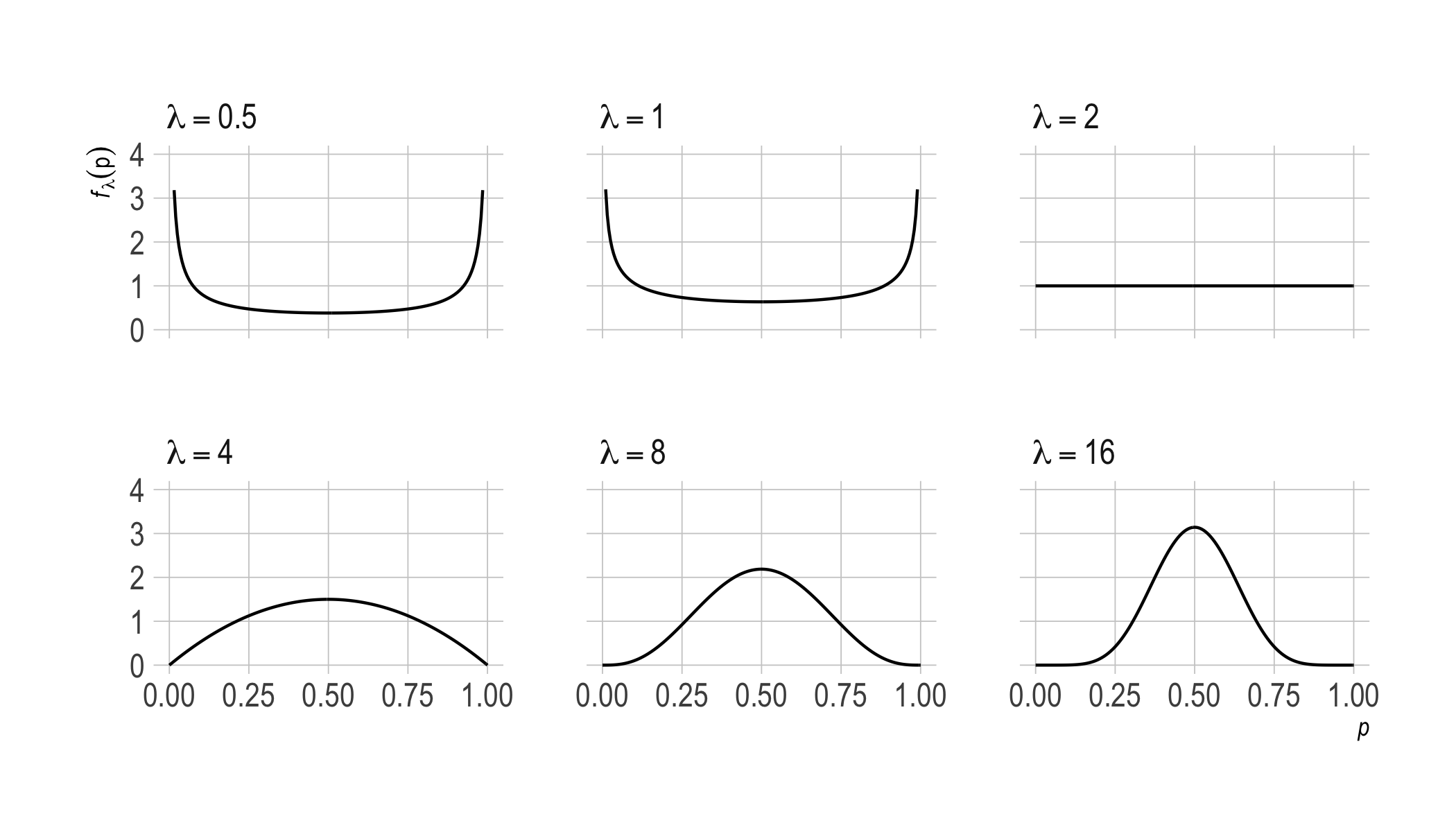
Notice how $\lambda = 2$ is a kind of inflection point. The plot goes from being concave up to concave down. When $\lambda < 2$, the prior is U-shaped. Then, as $\lambda$ grows above $2$, we approach a normal distribution centered on $1/ 2$.

So, when $\lambda < 2$, we start out pretty sure the coin is biased, though we don’t know in which direction. When $\lambda < 2$ we’re inclined to run with the observed frequency, whatever that is. If we observe a heads on the first toss, we’ll be pretty confident the next toss will land heads too. And the lower $\lambda$ is, the more confident we’ll be about that.

Whereas $\lambda > 2$ corresponds to an inclination to think the coin fair, or at least fair-ish. So it takes a while for the observed frequency to draw us away from our initial expectation of $1/ 2$. (Unless the observed frequency is itself $1/ 2$.)

That’s the intuitive picture we’re working towards. Let’s see how to get there.

Pseudo-observations

Notice that the Rule of Succession is the same as pretending we’ve already observed one heads and one tails, and then using the Straight Rule. A $3$rd toss landing heads would give us an observed frequency of $2/3$, precisely what the Rule of Succession gives when just $1$ toss has landed heads. If $k = n = 1$, then $$ \frac{k+1}{n+2} = \frac{2}{3}. $$ So, setting $\lambda = 2$ amounts to imagining we have $2$ observations already, and then using the observed frequency as the posterior probability.

Setting $\lambda = 4$ is like pretending we have $4$ observations already. If we have $2$ heads and $2$ tails so far, then a heads on the $5$th toss would make for an observed frequency of $3/5$. And this is the posterior probability the $\lambda$-continuum dictates for a single heads when $\lambda = 4$: $$ \frac{k + \lambda/2}{n + \lambda} = \frac{1 + 4/2}{1 + 4} = \frac{3}{5}. $$ In general, even values of $\lambda > 0$ amount to pretending we’ve already observed $\lambda$ flips, evenly split between heads and tails, and then using the observed frequency as the posterior probability.

This doesn’t quite answer our question, but it’s the key idea. We know that the uniform prior distribution gives rise to the posterior probabilities dictated by $\lambda = 2$. We want to know what prior distribution corresponds to other settings of $\lambda$. We see here that, for $\lambda = 4, 6, 8, \ldots$ the relevant prior is the same as the “pseudo-posterior” we would have if we updated the uniform prior on an additional $2$ “pseudo-observations”, or $4$, or $6$, etc.

So we just need to know what these pseudo-posteriors look like, and then extend the idea beyond even values of $\lambda$.

Pseudo-posteriors

Let’s write $S_n = k$ to mean that we’ve observed $k$ heads out of $n$ flips. We’ll use $p$ for the unknown, true probability of heads on each flip. Our uniform prior distribution is $f(p) = 1$ for $0 \leq p \leq 1$. We want to know what $f(p \given S_n = k)$ looks like.

In a previous post we derived a formula for this: $$ f(p \given S_n = k) = \frac{(n+1)!}{k!(n-k)!} p^k (1-p)^{n-k}. $$ This is the posterior distribution after observing $k$ heads out of $n$ flips, assuming we start with a uniform prior which corresponds to $\lambda = 2$. So, when we set $\lambda$ to a larger even number, it’s the same as starting with $f(p) = 1$ and updating on $S_{\lambda - 2} = \lambda/2 - 1$. We subtract $2$ here because $2$ pseudo-observations were already counted in forming the uniform prior $f(p) = 1$.

Thus the prior distribution $f_\lambda$ for a positive, even value of $\lambda$ is: $$ \begin{aligned} f_\lambda(p) &= f(p \given S_{\lambda - 2} = \lambda/2 - 1)\\
&= \frac{(\lambda - 1)!}{(\lambda/2 - 1)!(\lambda/2 - 1)!} p^{\lambda/2 - 1} (1-p)^{\lambda/2 - 1}. \end{aligned} $$ This prior generates the picture we started with for $\lambda \geq 2$.

As $\lambda$ increases, we move from a uniform prior towards a normal distribution centered on $p = 1/ 2$. This makes intuitive sense: the more we accrue evenly balanced observations, the more our expectations come to resemble those for a fair coin.

So, what about odd values of $\lambda$? Or non-integer values? To generalize our treatment beyond even values, we need to generalize our formula for $f_\lambda$.

The Beta Prior

Recall our formula for $f(p \given S_n = k)$: $$ \frac{(n+1)!}{k!(n-k)!} p^k (1-p)^{n-k}. $$ This is a member of a famous family of probability densities, the beta densities. To select a member from this family, we specify two parameters $a,b > 0$ in the formula: $$ \frac{1}{B(a,b)} p^{a-1} (1-p)^{b-1}. $$ Here $B(a,b)$ is the beta function, defined: $$ B(a,b) = \int_0^1 x^{a-1} (1-x)^{b-1} \dif x. $$ We showed that, when $a$ and $b$ are natural numbers, $$ B(a,b) = \frac{(a-1)!(b-1)!}{(a+b-1)!}. $$ To generalize our treatment of $f_\lambda$ beyond whole numbers, we first need to do the same for the beta function. We need $B(a,b)$ for all positive real numbers.

As it turns out, this is a matter of generalizing the notion of factorial. The generalization we need is called the gamma function, and it looks like this:

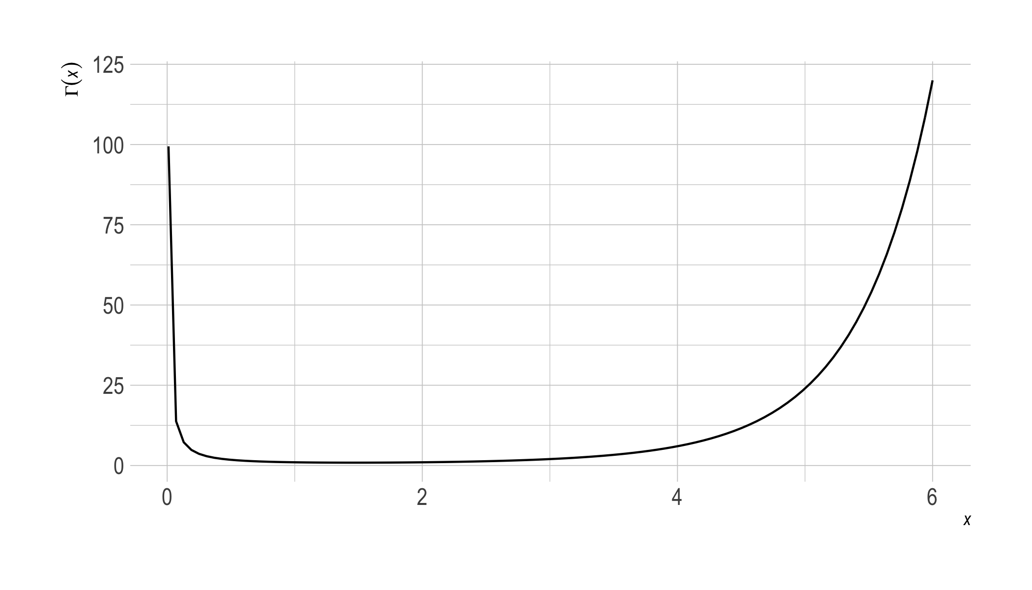
The formal definition is $$ \Gamma(x) = \int_0^\infty u^{x-1} e^{-u} \dif u. $$ The gamma function connects to the factorial function because it has the property: $$ \Gamma(x+1) = x\Gamma(x). $$ This entails, by induction, that $\Gamma(n) = (n-1)!$ for any natural number $n$.

In fact we can substitute gammas for factorials in our formula for the beta function: $$ B(a,b) = \frac{\Gamma(a)\Gamma(b)}{\Gamma(a+b)}. $$ Proving this formula would require a long digression, so we’ll take it for granted here.

Now we can now work with beta densities whose parameters are not whole numbers. For any $a, b > 0$, the beta density is $$ \frac{\Gamma(a + b)}{\Gamma(a)\Gamma(b)} p^{a-1} (1-p)^{b-1}. $$ We can now show our main result: setting $a = b = \lambda/2$ generates the $\lambda$-continuum.

From Beta to Lambda

We’ll write $X_{n+1} = 1$ to mean that toss $n+1$ lands heads. We want to show $$ \p(X_{n+1} = 1 \given S_n = k) = \frac{k + \lambda/2}{n + \lambda}, $$ given two assumptions.

The tosses are independent and identically distributed with probability $p$ for heads.
The prior distribution $f_\lambda(p)$ is a beta density with $a = b = \lambda/2$.

We start by applying the Law of Total Probability: $$ \begin{aligned} P(X_{n+1} = 1 \given S_n = k) &= \int_0^1 P(X_{n+1} = 1 \given S_n = k, p) f_\lambda(p \given S_n = k) \dif p\\
&= \int_0^1 p f_\lambda(p \given S_n = k) \dif p. \end{aligned} $$ Notice, this is the expected value of $p$, according to the posterior $f_\lambda(p \given S_n = k)$. To analyze it further, we use two facts proved below.

The posterior $f_\lambda(p \given S_n = k)$ is itself a beta density, but with parameters $k + \lambda/2$ and $n - k + \lambda/2$.
The expected value of any beta density with parameters $a$ and $b$ is $a/(a+b)$.

Thus $$ \begin{aligned} P(X_{n+1} = 1 \given S_n = k) &= \int_0^1 p f_\lambda(p \given S_n = k) \dif p \\
&= \frac{k + \lambda/2}{k + \lambda/2 + n - k + \lambda/2}\\
&= \frac{k + \lambda/2}{n + \lambda}. \end{aligned} $$ This is the desired result, we just need to establish Facts 1 and 2.

Fact 1

Here we show that, if $f(p)$ is a beta density with parameters $a$ and $b$, then $f(p \given S_n = k)$ is a beta density with parameters $k+a$ and $n - k + b$.

Suppose $f(p)$ is a beta density with parameters $a$ and $b$: $$ f(p) = \frac{1}{B(a, b)} p^{a-1} (1-p)^{b-1}. $$ We calculate $f(p \given S_n = k)$ using Bayes’ theorem: \begin{align} f(p \given S_n = k) &= \frac{f(p) P(S_n = k \given p)}{P(S_n = k)}\\
&= \frac{p^{a-1} (1-p)^{b-1} \binom{n}{k} p^k (1-p)^{n-k}}{B(a,b) P(S_n = k)}\\
&= \frac{\binom{n}{k}}{B(a,b) \p(S_n = k)} p^{k+a-1} (1-p)^{n-k+b-1} .\tag{1} \end{align} To analyze $\p(S_n = k)$, we begin with the Law of Total Probability: $$ \begin{aligned} P(S_n = k) &= \int_0^1 P(S_n = k \given p) f(p) \dif p\\
&= \int_0^1 \binom{n}{k} p^k (1-p)^{n-k} \frac{1}{B(a, b)} p^{a-1} (1-p)^{b-1} \dif p\\
&= \frac{\binom{n}{k}}{B(a, b)} \int_0^1 p^{a+k-1} (1-p)^{b+n-k-1} \dif p\\
&= \frac{\binom{n}{k}}{B(a, b)} B(k+a, n-k+b). \end{aligned} $$ Substituting back into Equation (1), we get: $$ f(p \given S_n = k) = \frac{1}{B(k+a, n-k+b)} p^{k+a-1} (1-p)^{n-k+b-1}. $$ So $f(p \given S_n = k)$ is the beta density with parameters $k + a$ and $n - k + b$.

Fact 2

Here we show that the expected value of a beta density with parameters $a$ and $b$ is $a/(a+b)$. The expected value formula gives: $$ \frac{1}{B(a, b)} \int_0^1 p p^{a-1} (1-p)^{b-1} \dif p\\
= \frac{\Gamma(a + b)}{\Gamma(a)\Gamma(b)} \int_0^1 p^a (1-p)^{b-1} \dif p. $$ The integrand look like a beta density, with parameters $a+1$ and $b$. So we multiply by $1$ in a form that allows us to pair it with the corresponding normalizing constant: $$ \begin{aligned} \begin{split} \frac{\Gamma(a + b)}{\Gamma(a)\Gamma(b)} & \int_0^1 p^a (1-p)^{b-1} \dif p \\
&= \frac{\Gamma(a + b)}{\Gamma(a)\Gamma(b)} \frac{\Gamma(a + 1)\Gamma(b)} {\Gamma(a + b + 1)}\int_0^1 \frac{\Gamma(a + b + 1)}{\Gamma(a + 1)\Gamma(b)} p^a (1-p)^{b-1} \dif p\\
&= \frac{\Gamma(a + b)}{\Gamma(a)\Gamma(b)} \frac{\Gamma(a + 1)\Gamma(b)} {\Gamma(a + b + 1)}. \end{split} \end{aligned} $$ Finally, we use the the property $\Gamma(a+1) = a \Gamma(a)$ to obtain: $$ \frac{\Gamma(a + b)}{\Gamma(a)\Gamma(b)} \frac{a\Gamma(a)\Gamma(b)} {(a+b) \Gamma(a + b)} = \frac{a} {a+b}. $$

Picturing It

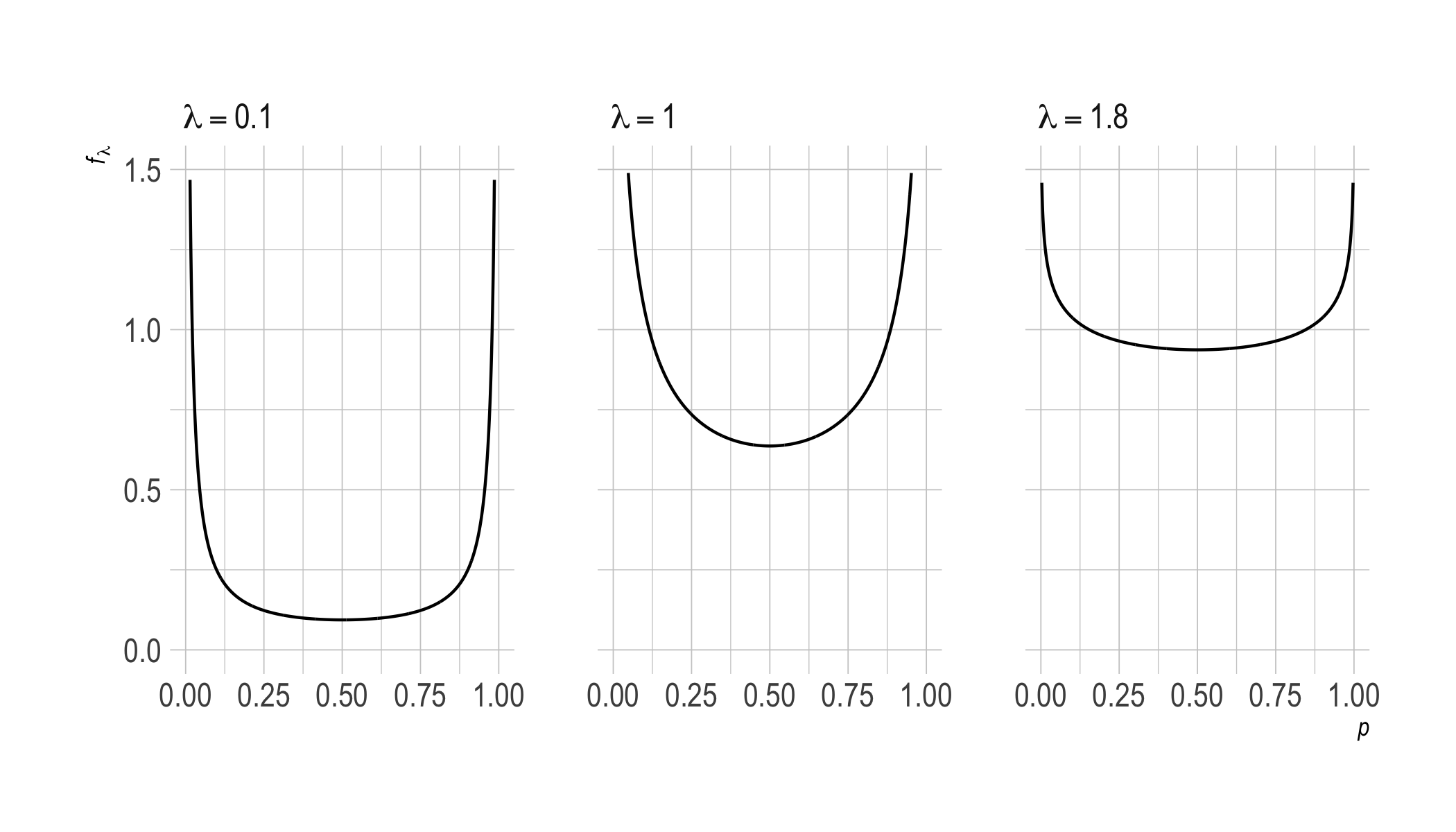
What do our priors corresponding to $\lambda < 2$ look like? Above we saw that they’re U-shaped, approaching a flat line as $\lambda$ increases. Here’s a closer look:

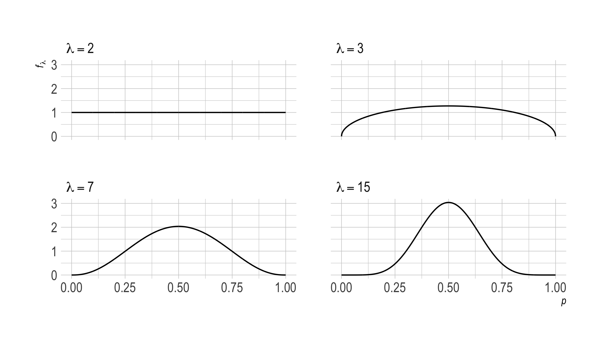
We can also look at odd values $\lambda \geq 2$ now, where the pattern is the same as we observed previously.

What About Zero?

What about when $\lambda = 0$? This is a permissible value on the $\lambda$-continuum, giving rise to the Straight Rule as we’ve noted. But it doesn’t correspond to any beta density. The parameters would be $a = b = \lambda/2 = 0$. Whereas we require $a, b > 0$, since the integral $$ \int_0^1 p^{-1}(1-p)^{-1} \dif p $$ diverges.

In fact no prior can agree with the Straight Rule. At least, not on the standard axioms of probability. The Straight Rule requires $\p(HH \given H) = 1$, which entails $\p(HT \given H) = 0$. By the usual definition of conditional probability then, $\p(HT) = 0$. Which means $\p(HTT \given HT)$ is undefined. Yet the Straight Rule says $\p(HTT \given HT) = 1/ 2$.

We can accommodate the Straight Rule by switching to a nonstandard axiom system, where conditional probabilities are primitive, rather than being defined as ratios of unconditional probabilities. This is approach is sometimes called “Popper–Rényi” style probability.

Alternatively, we can stick with the standard, Kolmogorov system and instead permit “improper” priors: prior distributions that don’t integrate to $1$, but which deliver posteriors that do.

Taking this approach, the beta density with $a = b = 0$ is called the Haldane prior. It’s sometimes regarded as “informationless,” since its posteriors just follow the observed frequencies. But other priors, like the uniform prior, also have some claim to representing perfect ignorance. The Jeffreys prior, which is obtained by setting $a = b = 1/ 2$ (so $\lambda = 1$), is another prior with a similar claim.

That multiple priors can make this claim is a reminder of one of the great tragedies of epistemology: the problem of priors.

Acknowledgments

I’m grateful to Boris Babic for reminding me of the beta-lambda connection. For more on beta densities I recommend the videos at stat110.net.

The Beta Prior and the Lambda Continuum