There are four ways things can turn out with two flips of a coin: $$ HH, \quad HT, \quad TH, \quad TT.$$ If we know nothing about the coin’s tendencies, we might assign equal probability to each of these four possible outcomes: $$ Pr(HH) = Pr(HT) = Pr(TH) = Pr(TT) = 1/ 4. $$ But from another point of view, there are primarily three possibilities. If we ignore order, the possible outcomes are $0$ heads, $1$ head, or $2$ heads. So we might instead assign equal probability to these three outcomes, then divide the middle $1/ 3$ evenly between $HT$ and $TH$: $$ Pr(HH) = 1/3 \qquad Pr(HT) = Pr(TH) = 1/6 \qquad Pr(TT) = 1/ 3. $$

This two-stage approach may seem odd. But it’s actually friendlier from the point of view of inductive reasoning. On the first scheme, a heads on the first toss doesn’t increase the probability of another heads. It stays fixed at $1/ 2$: $$ \newcommand{\p}{Pr} \newcommand{\given}{\mid} \renewcommand{\neg}{\mathbin{\sim}} \renewcommand{\wedge}{\mathbin{\text{&}}} \p(HH \given H) = \frac{1/ 4}{1/ 4 + 1/ 4} = \frac{1}{2}. $$ Whereas it does increase on the second strategy, from $1/ 2$ to $2/ 3$: $$ \p(HH \given H) = \frac{1/ 3}{1/ 3 + 1/ 6} = \frac{2}{3}. $$ The two-stage approach thus learns from experience, where the single-step division is skeptical about induction.

This holds true as we increase the number of flips. If we do three tosses for example, we’ll find that $\p(HHH \given HH) = 3/ 4$ on the two-stage analysis. Whereas this probability stays stubbornly fixed at $1/ 2$ on the first approach. It won’t budge no matter how many heads we observe, so we can’t learn anything about the coin’s bias this way.

This is the difference between Carnap’s famous account of induction, from his 1950 book Logical Foundations of Probability, and the account he finds in Wittgenstein’s Tractatus. ¹ Although Carnap had actually been scooped by W. E. Johnson, who worked out a similar analysis about $25$ years earlier.

This is a short explainer on some key elements of inductive logic worked out by Johnson and Carnap and the place of those ideas in the story of inductive logic.

• PDF version here

States & Structures

Carnap calls a fine-grained specification like $TH$ a state-description. The coarser grained “$1$ head” is a structure-description. A state-description specifies which flips land heads, and which tails. While a structure-description specifies how many land heads and tails, without necessarily saying which.

It needn’t be coin flips landing heads or tails, of course. The same ideas apply to any set of objects or events, and any feature they might have or lack.

Suppose we have two objects $a$ and $b$, each of which might have some property $F$. Working for a moment as Carnap did, in first-order logic, here is an example of a structure-description: $$ (Fa \wedge \neg Fb) \vee (\neg Fa \wedge Fb). $$ But this isn’t a state-description, since it doesn’t specify which object has $F$. It only says how many objects have $F$, namely $1$. One of the disjuncts alone would be a state-description though: $$ Fa \wedge \neg Fb. $$

Carnap’s initial idea was that all structure-descriptions start out with the same probability. These probabilities are then divided equally among the state-descriptions that make up a structure-description.

For example, if we do three flips, there are four structure-descriptions: $0$ heads, $1$ head, $2$ heads, and $3$ heads. Some of these have only one state-description. For example, there’s only one way to get $0$ heads, namely $TTT$. So $$ \p(TTT) = 1/ 4. $$ But others have multiple state-descriptions. There are three ways to get $1$ head for example, so we divide $1/ 4$ between them: $$ \p(HTT) = \p(THT) = \p(TTH) = 1/ 12. $$

The effect is that more homogeneous sequences start out more probable. There’s only one way to get all heads, so the $HH$ state-description inherits the full probability of the corresponding “$2$ heads” structure-description. But a $50$-$50$ split has multiple permutations, each of which inherits only a portion of the same quantum of probability. A heterogeneous sequence of heads and tails thus starts out less probable than a homogeneous one.

That’s why the two-stage analysis is induction-friendly. It effectively builds Hume’s “uniformity of nature” assumption into the prior probabilities.

The Rule of Succession

The two-stage assignment also yields a very simple formula for induction: Laplace’s famous Rule of Succession. (Derivation in the Appendix.)

The Rule of Succession

Given $k$ heads out of $n$ observed flips, the probability of heads on a subsequent toss is $$\frac{k+1}{n+2}.$$

Laplace arrived at this rule about $150$ years earlier by somewhat different means. But there is a strong similarity.

Laplace supposed that our coin has some fixed, but unknown, chance $p$ of landing heads on each toss. Suppose we regard all possible values $0 \leq p \leq 1$ as equally likely.² If we then update our beliefs about the true value of $p$ using Bayes’ theorem, we arrive at the Rule of Succession. (Proving this is a bit involved. Maybe I’ll go over it another time.)

The two-stage way of assigning prior probabilities is essentially the same idea, just applied in a discrete setting. By treating all structure-descriptions as equiprobable, we make all possible frequencies of heads equiprobable. This is a discrete analogue of treating all possible values of $p$ as equiprobable.

The Continuum of Inductive Methods

Both Johnson and Carnap eventually realized that the two methods of assigning priors we’ve considered are just two points on a larger continuum.

The $\lambda$ Continuum

Given $k$ heads out of $n$ observed flips, the probability of heads on a subsequent toss is $$\frac{k + \lambda/2}{n + \lambda},$$ for some $\lambda$ in the range $0 \leq \lambda \leq \infty$.

What value should $\lambda$ take here? Notice we get the Rule of Succession if $\lambda = 2$. And we get inductive skepticism if we let $\lambda$ approach $\infty$. For then $k$ and $n$ fall away and the ratio converges to $1/ 2$, no matter what $k$ and $n$ are.

If we set $\lambda = 0$, we get a formula we haven’t discussed yet: $k/n$. Reichenbach called this the Straight Rule. (In modern statistical parlance it’s the “maximum likelihood estimate.”)³

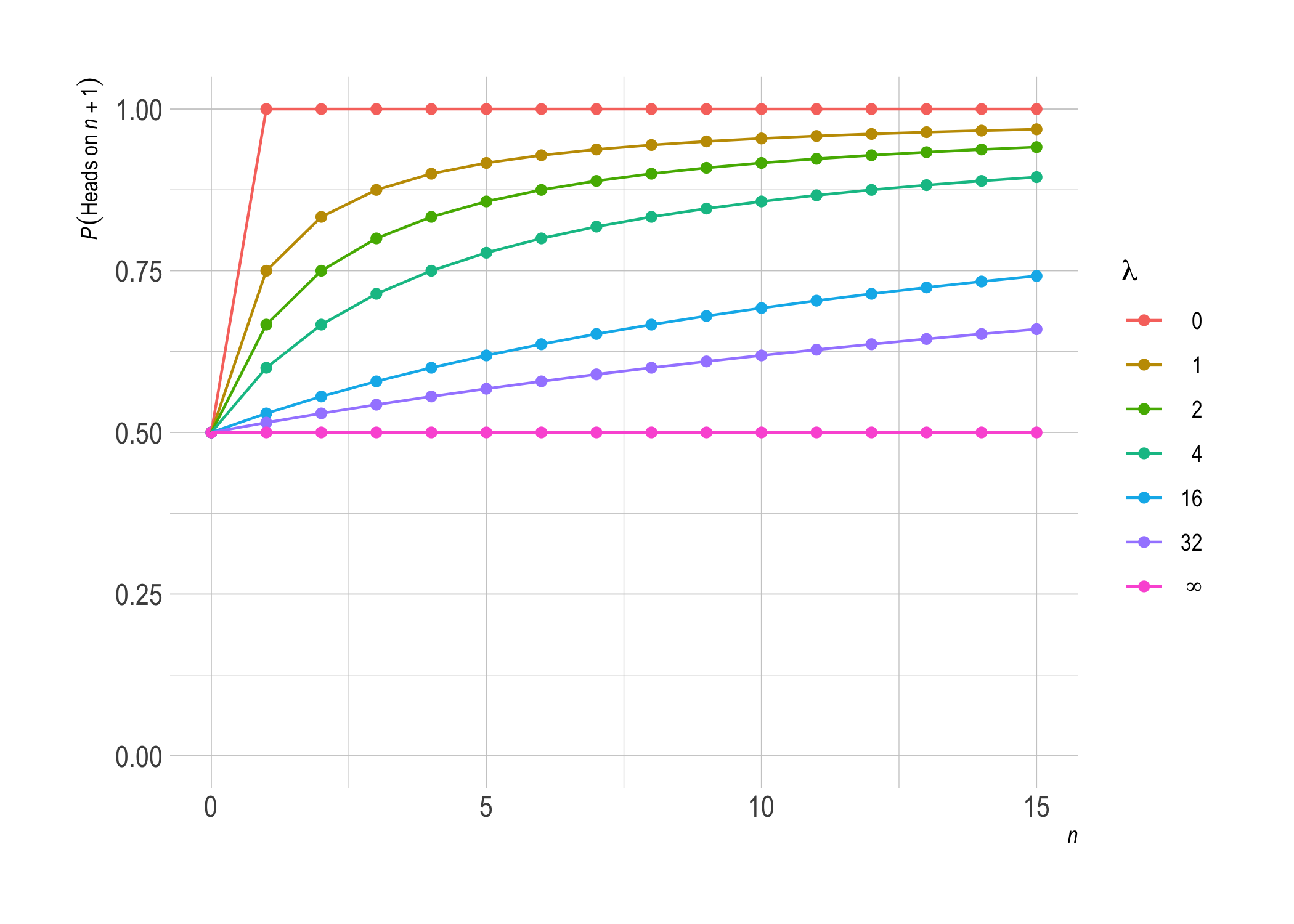
The overall pattern is: the higher $\lambda$, the more “cautious” our inductive inferences will be. A larger $\lambda$ means less influence from $k$ and $n$: the probability of another heads stays closer to the initial value of $1/ 2$. In the extreme case where $\lambda = \infty$, it stays stuck at exactly $1/ 2$ forever.

A low value of $\lambda$, on the other hand, will make our inferences more ambitious. In the extreme case $\lambda = 0$, we jump immediately to the observed frequency. Our expectation about the next toss is just $k/n$, the frequency we’ve observed so far. If we’ve observed only one flip and it was heads ($k = n = 1$), we’ll be certain of heads on the second toss! ⁴

We can illustrate this pattern in a plot. First let’s consider what happens if the coin keeps coming up heads, i.e. $k = n$. As $n$ increases, various settings of $\lambda$ behave as follows.

Now suppose the coin only lands heads every third time, so that $k \approx n/3$.

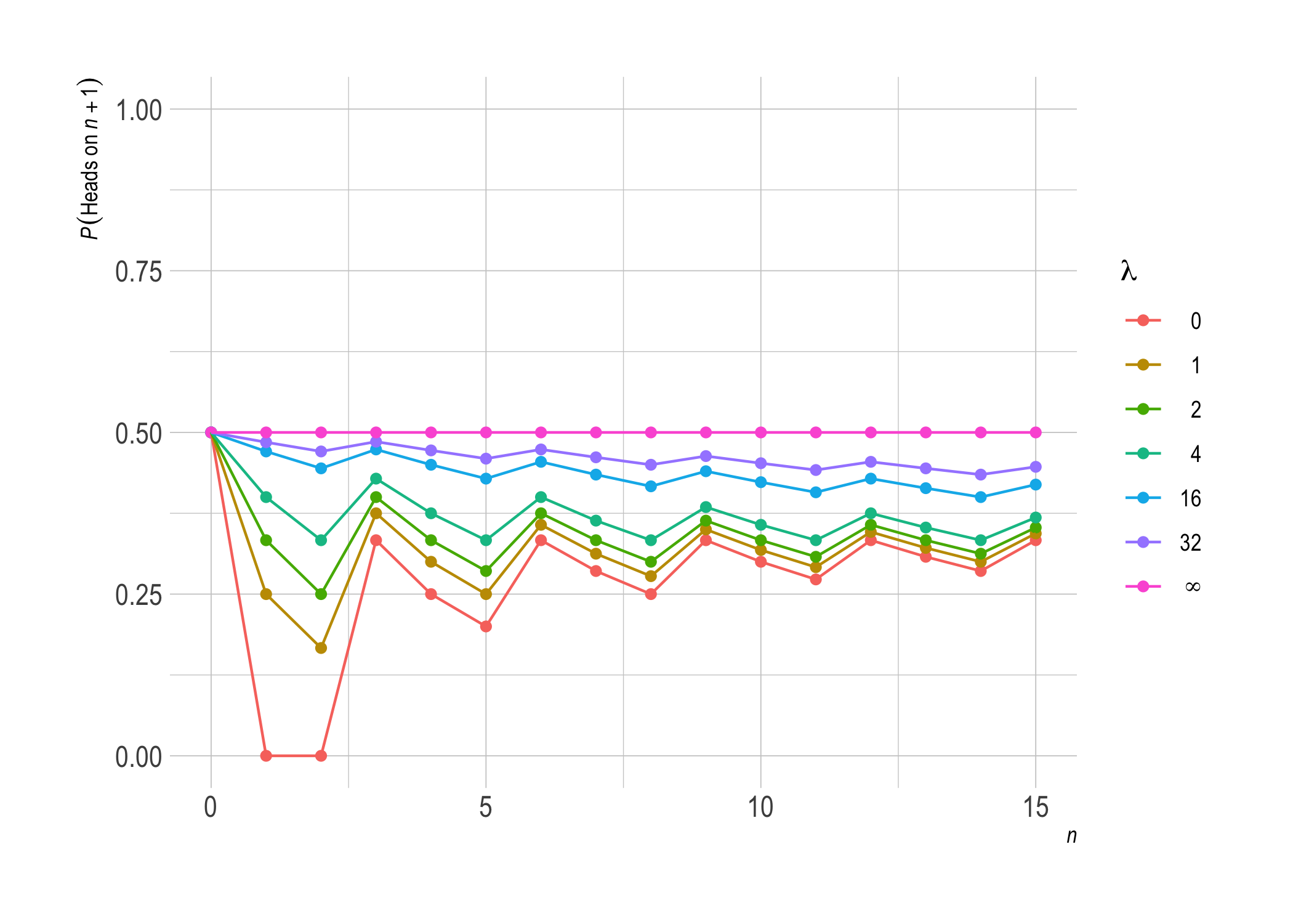
Notice how lower settings of $\lambda$ bounce around more here before settling into roughly $1/ 3$. Higher settings approach $1/ 3$ more steadily, but they take longer to get there.

Carnap’s Program

Johnson and Carnap went much further, and others since have gone further still. For example, we can include more than one predicate, we can use relational predicates, and much more.

But philosophers aren’t too big on this research program nowadays. Why not?

Choosing $\lambda$ is one issue. Once we see that it’s more than a binary choice, between inductive optimism and skepticism, it’s hard to see why we should plump for any particular value of $\lambda$. We could set $\lambda = 2$, or $\pi$, or $42$. By what criterion could we make this choice? No clear answer emerged from Carnap’s program.

Another issue is Goodman’s famous grue puzzle. Suppose we trade our coin flips for emeralds. We might replace the heads/tails dichotomy with green/not-green then. But we could instead replace it with grue/not-grue. The prescriptions of our inductive logic depend on our choice of predicate—on the underlying language to which we apply our chosen value of $\lambda$.

So the Johnson/Carnap system doesn’t provide us with rules for inductive reasoning, more a framework for formulating such rules. We have to decide which predicates should be projectible by choosing the underlying language. And then we have to decide how projectible they should be by choosing $\lambda$. Only then does the framework tell us what conclusions to draw from a given set of observations.

Personally, I still find the framework useful. It provides a lovely way to express informal ideas more rigorously. In it we can frame questions about induction, skepticism, and prior probabilities with lucidity.

I also like it as a source of toy models. For example, I might test when a given claim about induction holds and when it doesn’t, by playing with different incarnations of $\lambda$.

The framework’s utility is thus a lot like that of its deductive cousins. Compare Timothy Williamson’s use of modal logic to create models of Gettier cases, for example, or his model of improbable knowledge.

Even in deductive logic, we only get as much out as we put in. We have to choose our connectives in propositional logic, our accessibility relation in modal logic, etc. But a flexible system like possible-world frames still has its uses. We can use it to explore philosophical options and their interconnections.

Further Readings

For more on this topic I suggest the following readings.

• Inductive Logic, by Branden Fitelson
• Carnap on Probability and Induction, by Sandy Zabell
• The IEP entry on Confirmation and Induction, by Franz Huber
• The SEP entry on Inductive Logic, by James Hawthorne
• Pure Inductive Logic, by Jeffrey Paris and Alena Vencovská

If you want to see how Johnson and Carnap’s two-stage assignment of priors yields the Rule of Succession, check out the Appendix.

Appendix: Deriving the Rule of Succession

To derive the Rule of Succession from the two-stage assignment of priors, we need two key formulas.

1. The prior probability of a particular sequence with $k$ heads out of $n$ flips.
2. The prior probability of the same initial sequence, followed by one more heads.

The first quantity is the probability of getting $k$ heads out of $n$ flips, regardless of order, divided by the number of ways to get $k$ heads out of $n$ flips. The number of ways to get $k$ heads out of $n$ flips is called the binomial coefficient. It’s written $\binom{n}{k}$, and there’s a nice formula for calculating it: $$ \binom{n}{k} = \frac{n!}{(n-k)!k!}. $$ Since a sequence of $n$ flips can feature anywhere from $0$ to $n$ heads, there are $n+1$ structure descriptions, each with probability $1/(n+1)$. Thus the probability of a specific state-description with $k$ heads out of $n$ flips is \begin{align} \frac{1}{(n+1)\binom{n}{k}} &= \frac{1}{(n+1) \frac{n!}{(n-k)!k!}}\\
&= \frac{(n-k)!k!}{(n+1)!}.\tag{1} \end{align}

The second probability we need is for the same initial sequence, but with an additional heads on the next toss. That’s a sequence with $k+1$ heads out of $n+1$ tosses. There are $n+2$ structure descriptions now, each with probability $1/(n+2)$. So the probability in question is \begin{align} \frac{1}{(n+2)\binom{n+1}{k+1}} &= \frac{1}{(n+2) \frac{(n+1)!}{(n-k)!(k+1)!}}\\
&= \frac{(n-k)!(k+1)!}{(n+2)!}.\tag{2} \end{align}

Now, to get the conditional probability we’re after, we take the ratio of the second probability $(2)$ over the first probability $(1)$: $$ \begin{aligned} \frac{ \frac{(n-k)!(k+1)!}{(n+2)!} }{ \frac{(n-k)!k!}{(n+1)!} } &= \frac{(n-k)!(k+1)!}{(n+2)!} \frac{(n+1)!}{(n-k)!k!} \\
&= \frac{k+1}{n+2}. \end{aligned} $$ This agrees with the rule of succession, as desired.

So far though, we’ve only shown the rule of succession for a specific, observed sequence. We’ve shown that $\p(HTHH \given HTH) = 3/ 4$, for example. But what if we don’t know the particular sequence so far? Maybe we only know there were $2$ heads out of $3$ tosses. Shouldn’t we still be able to derive the same result?

We can, with the help of a relevant theorem of probability: if $\p(A \given B) = \p(A \given C)$, and $B$ and $C$ are mutually exclusive, then $$ \p(A \given B \vee C) = \p(A \given B) = \p(A \given C). $$ In our case $A$ specifies heads on flip $n+1$, while $B$ and $C$ each specify some sequence for flips $1$ through $n$. Although these sequences feature the same number of heads and tails, $B$ and $C$ specify different orderings. So they’re mutually exclusive.

We’ve already shown that $$ \p(A \given B) = \frac{k+1}{n+2} = \p(A \given C). $$ So we just have to verify the theorem: $$ \begin{aligned} \p(A \given B \vee C) &= \frac{\p(A \wedge (B \vee C))}{\p(B \vee C)}\\
&= \frac{\p(A \wedge B) + \p(A \wedge C)}{\p(B \vee C)}\\
&= \frac{\p(A \given B)\p(B) + \p(A \given C)\p( C)}{\p(B \vee C)}\\
&= \frac{\p(A \given B) \left( \p(B) + \p( C) \right)}{\p(B \vee C)}\\
&= \p(A \given B). \end{aligned} $$ By applying this formula repeatedly to a disjunction of state-descriptions, we get the conditional probability on the structure description of interest.