It’s only natural to place less trust in the judgment of those who disagree with you. After all, from your point of view, those people are mistaken! And making mistakes is a sign of incompetence.

This kind of distrust is actually baked into a number of models in social epistemology (for example: here, here, and here). I gave an argument against the rationality of one such model in a previous post. But the argument doesn’t really depend on the details of the model; any rule that discounts evidence reported by a source you disagree with will run into the same problem.

A policy of distrusting those who disagree with you is also reminiscient of some classic issues in the debate about peer disagreement. So I think it’s worth getting clear on the extent to which such distrust makes sense, and trying to understand, when it goes wrong, why it goes wrong. In this post I’ll take a first stab at a diagnosis.

One Model of Competence

Suppose you and a friend are investigating some hypothesis, $H$. If $H$ is true, then experiments on $H$ yield a “positive” result with some fixed probability $p$, whereas if $H$ is false, the “positive” rate is instead some lower value $q$. So we can think of $H$ as saying that some coin has bias $p$, and $\n{H}$ as saying the bias is instead $q$.

We’ll understand your friend’s competence as their reliability at recognizing positive evidence as positive, and negative evidence as negative. In other words, it’s the probability that they’ll correctly identify a heads as heads, and a tails as tails.

Now, imagine you and your friend each go off and do some independent experimenting on $H$. It seems plausible that, when you reconvene, you should find yourselves with similar opinions, if your friend is competent. Of course, it’s possible that one of you will get an unlucky batch of misleading evidence, and end up with the wrong view of $H$ despite being perfectly competent. But the more evidence you gather, the more likely it is that you’ll converge on the truth about $H$—if, again, your friend is competent.

So shouldn’t you question your friend’s competence if they come back with a different opinion than yours? And suspect them more the more their opinion differs?

Curiously, no. At least, not in this model. The figure below shows how your estimate of your friend’s competence varies with the number of “heads” they claim to have encountered, in one instance of the model.

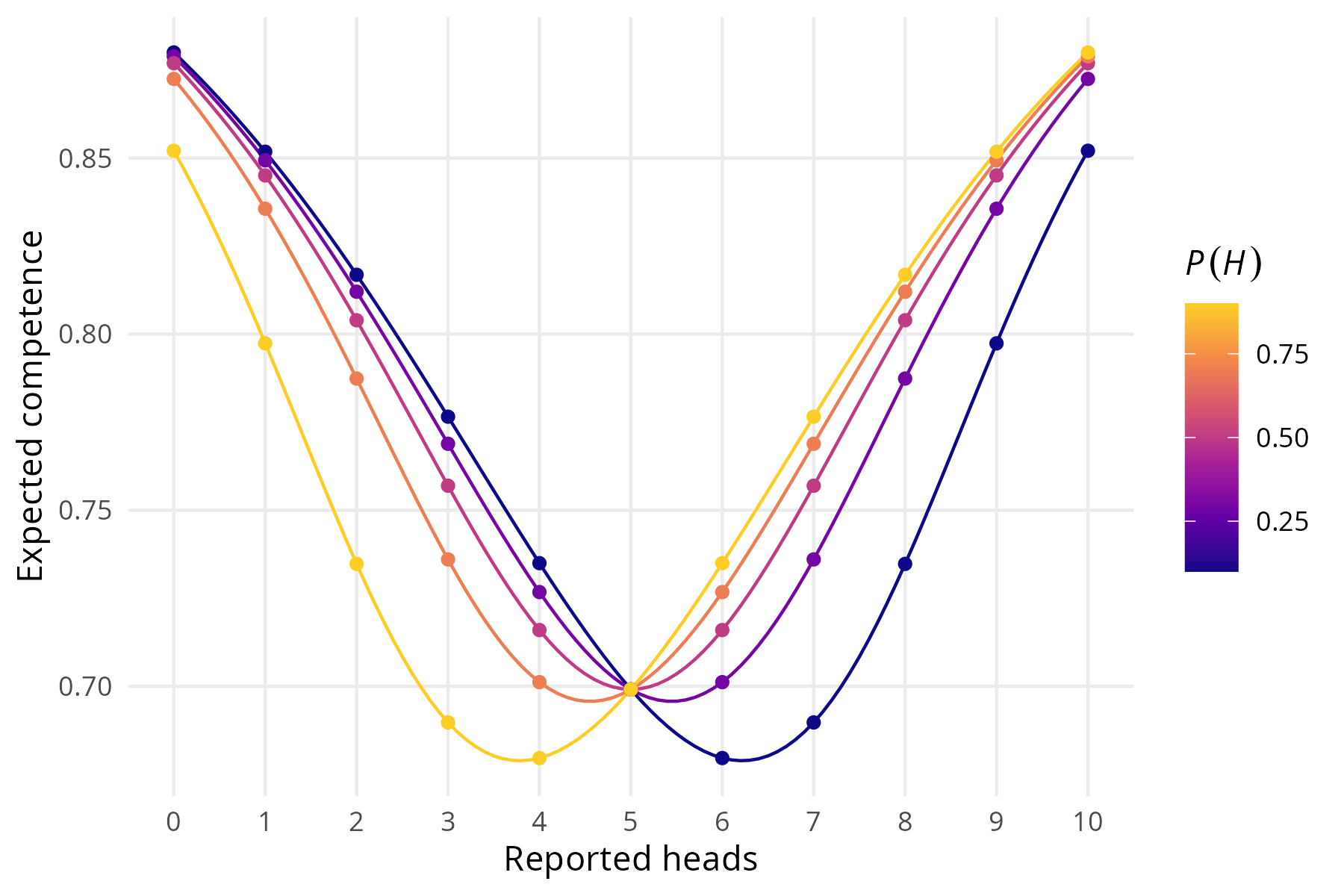
In this instance:

• the coin’s bias is either $p=¾$ or $q=¼$,
• your friend does $10$ tosses, and
• they might be perfectly competent ($C = 1$), perfectly incompetent ($C = ½$), or anything in between. All possibilities in this range are equally probable to start.

The exact result depends on your $P(H)$, but the pattern is the same across various opinions you might hold about $H$: the more extreme your friend’s opinion, the higher you’ll rate their competence.

Understanding the Result

That’s an odd result, so let’s see if we can understand how it arises.

To fix ideas, suppose for a moment that $H$ is true, so the coin has bias $p=¾$. If your friend is perfectly competent ($C=1$), then the most likely outcome is they think they observe $7$ or $8$ heads. Whereas, if they’re perfectly incompetent ($C=½$), they’ll probably claim to get around $5$ heads.

But that’s the wrong comparison to make! What matters is not where each likelihood function has its peak, but where the ratio of the two likelihood functions has its maximum. That tells us where the competence and incompetence hypotheses have the starkest contrast, and thus where the strongest evidence for discriminating between them lies.

Now, the more “heads” your friend reports, the more this ratio increases. Think about it this way: each heads is $1.5$ times more likely given competence than it is given incompetence. Each time the coin lands, there’s only a $½$ chance they’ll see it as heads if they’re incompetent, as compared with a $¾$ chance if they’re competent. So each time they call “heads”, the odds of the competent hypothesis increase by a factor of $1.5$.

That’s all assuming the bias is $p=¾$, which of course you don’t know. If instead the bias is $q=¼$, the story inverts: the competence hypothesis gets a $1.5\times$ boost each time your friend calls “tails” instead. But, while the evidence for competence is strongest at the opposite extreme in this case, it is still strongest at the extreme.

You might think that, if you don’t know which case you’re in—$p=¾$ or $q=¼$—then this extremizing tendency will get washed out when you average the two cases according to your probability for each. But no, as the following figure shows. Even if you’re entirely uncertain which is the true bias, with $P(H) = P(\n{H}) = ½$, the starkest contrast is still at the extremes:

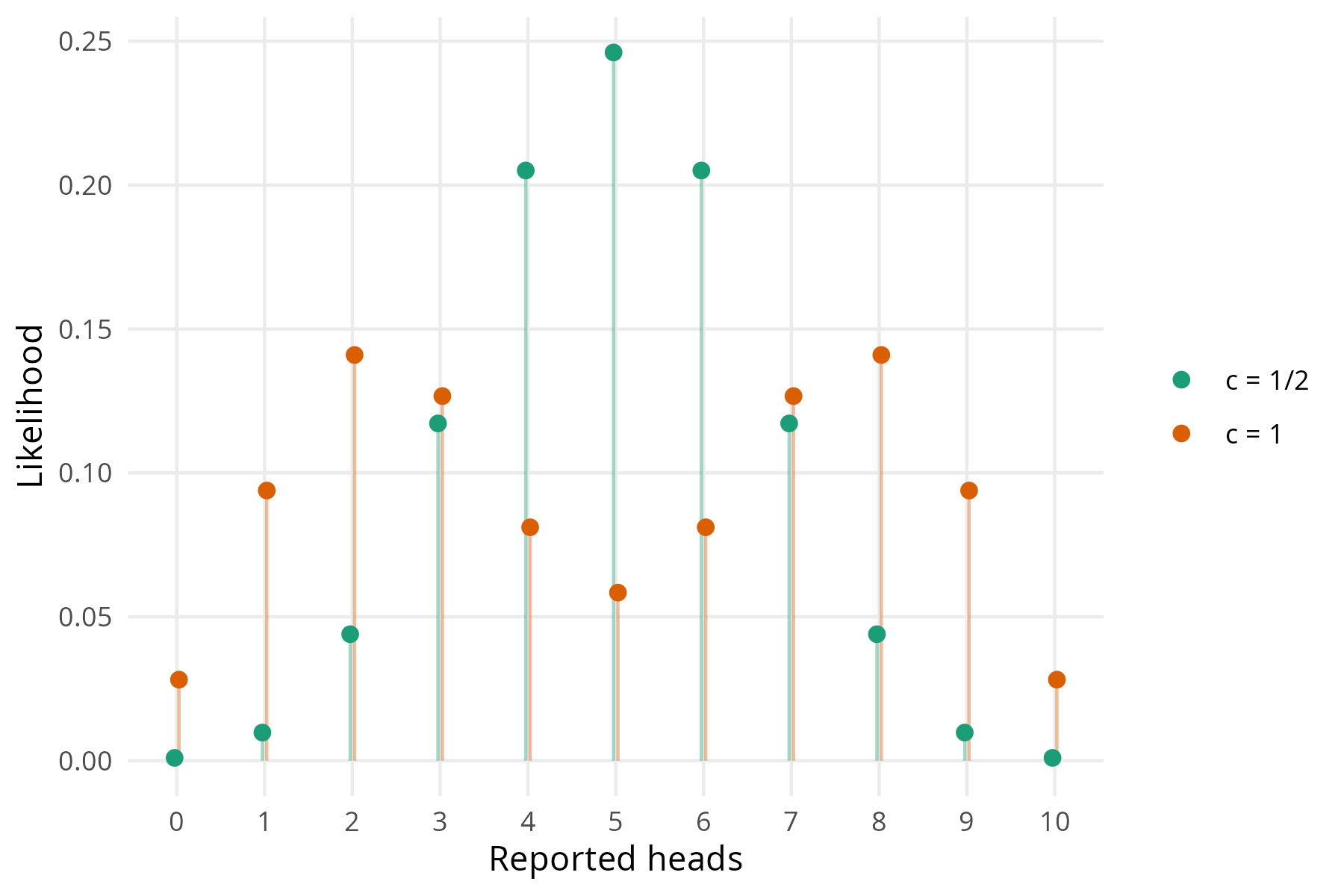
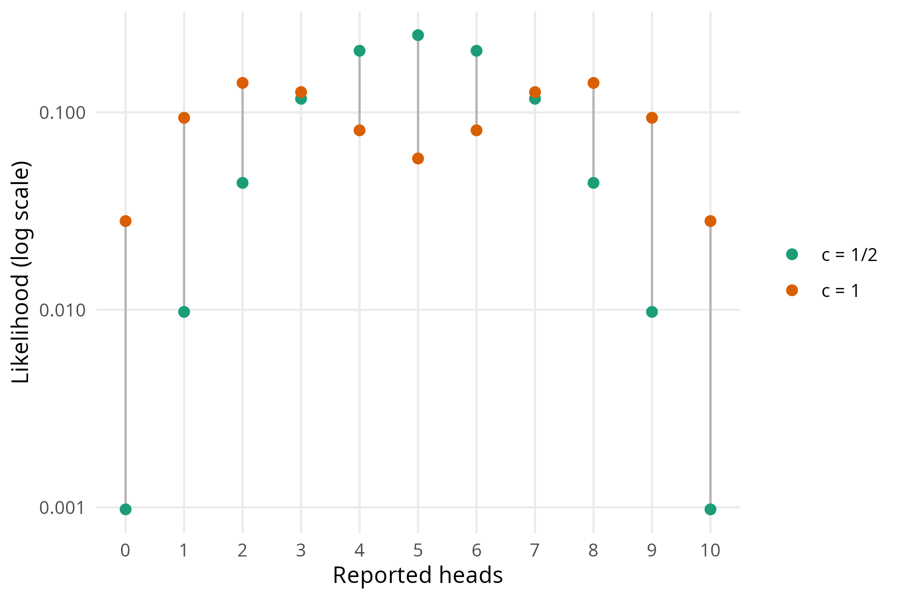
A bit confusingly, that’s not where the biggest difference is between the likelihoods of our two hypotheses about your friend’s competence. So it may help to view things on a log scale. Then the differences in the plot tell us where the likelihood ratio is largest, namely at the extremes:

A Diagnosis

So our diagnosis, at least in the case of this model, is as follows. The temptation to think that distrust tracks difference of opinion comes from a confusion between two questions.

1. What outcome is most expected if your friend is competent?
2. What outcome has the greatest contrast in what we expect from competence vs. incompetence?

That question (2) is what matters is a classic Bayesian moral, the law of likelihood. Relying instead on question (1) is a fallacy Elliott Sober dubs probabilistic modus tollens. “If my friend is competent, they should end up with an opinion similar to mine; they haven’t; so they’re probably not competent.” Tempting, but unBayesian.

Getting More Realistic

Of course, that’s just one model, and it’s unrealistic in a number of ways. For one thing, it treats incompetence as random noise: on this model, an incompetent person treats positive and negative evidence identically, misreading both at the same rate. But, realistically, people misinterpret evidence and arguments in more systematic and biased ways, like wishful thinking.

So, a more realistic model would be one where your friend has a preference for $H$, and thus tends to see tails as heads more often than the other way around. Or, maybe, they have no initial preference, but as the data come in, they tend to interpret new data in line with whichever hypothesis has been favoured by the data so far.

I’ll try to work out the details of this kind of variation if I get the time. Meanwhile, here’s the math on the naive model we used here.

The Gory Details

Recall the model’s assumptions:

• A coin has one of two possible biases, $p$ or $q$.
• Your friend flips the coin some fixed number of times, $n$.
• Their competence level is some probability, $C \sim \textrm{Uniform}(a,b)$.
  • They perceive each toss correctly with probability $C$, otherwise they perceive the opposite result.
• At the end, they report how many heads they think they observed, $X$.

Under these assumptions, we can analyze the expected value of their competence given their report as follows: \begin{align} \E [ C \mid X=k ] &= \int_a^b c \, f(c \mid k) \d{c} \\
&= \int_a^b c \, \frac{ f( c) \, P(k \mid c) }{ P(k) } \d{c} \\
&= \frac{ \int_a^b c \, f( c) \, P(k \mid c) \d{c} }{ P(k) } \\
&= \frac{ \int_a^b c \, f( c) \, P(k \mid c) \d{c} }{ \int_a^b f( c) \, P(k \mid c) \d{c} } \\
&= \frac{ \int_a^b c \, P(k \mid c) \d{c} }{ \int_a^b P(k \mid c) \d{c} }. \end{align} Now, assuming $H$ and $c$ are independent, \begin{align} P(k \mid c) &= P(H) P(k \mid H, c) + P(\n{H}) P(k \mid \n{H}, c). \end{align} And if we define \begin{align} \rho(c, \theta) &= c \theta + (1-c)(1-\theta), \\
\beta(x) &= x^k (1-x)^{n-k}, \end{align} then we can express the conditional probabilities here as: \begin{align} P(k \mid H, c) &= \binom{n}{k} \rho(c, p)^k (1 - \rho(c, p))^{n-k} \\
&= \binom{n}{k} \beta(\rho(c, p)), \\
P(k \mid \n{H}, c) &= \binom{n}{k} \rho(c, q)^k (1 - \rho(c, q))^{n-k} \\
&= \binom{n}{k} \beta(\rho(c, q)). \end{align} Returning now to our analysis of $\E[C \mid X = k]$: \begin{align} \E [ C \mid X = k ] &= \frac{ \int_a^b c \, P(k \mid c) \d{c} }{ \int_a^b P(k \mid c) \d{c} } \\
&= \frac{ \int_a^b \left[c \, P(H) P(k \mid H, c) + c \, P(\n{H}) P(k \mid \n{H}, c) \right] \d{c} }{ \int_a^b \left[ P(H) P(k \mid H, c) + P(\n{H}) P(k \mid \n{H}, c) \right] \d{c} } \\
&= \frac{ P(H) \int_a^b c \, \beta(\rho(c, p)) \d{c} + P(\n{H}) \int_a^b c \, \beta(\rho(c, q)) \d{c} }{ P(H) \int_a^b \beta(\rho(c, p)) \d{c} + P(\n{H}) \int_a^b \beta(\rho(c, q)) \d{c} }. \end{align}

This is something we can express straightforwardly in code, and fixing $(p, q, a, b) = (¾, ¼, ½, 1)$, we get the first figure above.

We also focused on the special cases $C=½$ and $C=1$. Here, $$ \rho(c, \theta) = \begin{cases} ½ & \textrm{ if } c = ½, \\
\theta & \textrm{ if } c = 1, \end{cases} $$ so \begin{align} P(k \mid C=½) &= \binom{n}{k} (½)^n, \\
P(k \mid C=1) &= \binom{n}{k} \left[P(H) \, p^k (1-p)^{n-k} + P(\n{H})\, q^k (1-q)^{n-k}\right]. \end{align} These formulas give us the second and third figures above, assuming $P(H) = P(\n{H}) = ½$.