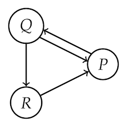
If you look at the little network diagram below, you’ll probably agree that $P$ is the most “central” node in some intuitive sense.

This post is about using a belief’s centrality in the web of belief to give a coherentist account of its justification. The more central a belief is, the more justified it is.

But how do we quantify “centrality”? The rough idea: the more ways there are to arrive at a proposition by following inferential pathways in the web of belief, the more central it is.

Since we’re coherentists today (for the next 10 minutes, anyway), cyclic pathways are allowed here. If we travel $P \rightarrow Q \rightarrow R \rightarrow P$, that counts as an inferential path leading to $P$. And if we go around that cycle twice, that counts as another such pathway.

You might think this just wrecks the whole idea. Every node has infinitely many such pathways leading to it, after all. By cycling around and around we can come up with literally any number of pathways ending at a given node.

But, by examining how these pathways differ in the limit, we can differentiate between more and less central nodes/beliefs. We can thus clarify a sense in which $P$ is most central, and quantify that centrality. We can even use that quantity to answer a classic objection to coherentism leveled by Klein & Warfield (1994).

As a bonus, we can do all this without ever giving an account of what makes a corpus of beliefs “coherent.” This flips the script on a lot of contemporary formal work on coherentism.¹ Because coherentism is holistic, you might think it has to evaluate the coherence of a whole corpus first, before it can assess the individual members.² But we’ll see this isn’t so. $$ \newcommand\T{\intercal} \newcommand{\A}{\mathbf{A}} \renewcommand{\v}{\mathbf{v}} $$

Counting Pathways

Our idea is to count how many paths there are leading to $P$ vs. other nodes. We start with paths of length $1$, then count paths of length $2$, then length $3$, and so on. As we count longer and longer paths, each node’s count approaches infinity.

But not their relative ratios! If, at each step, we divide the number of paths ending at $P$ by the number of all paths, this ratio converges.

To find its limit, we represent our graph numerically. A graph can be represented in a table, where each node corresponds to a row and column. The columns represent “sources” and the rows represent “targets.” We put a $1$ where the column node points to the row node, otherwise we put a $0$.

	$P$	$Q$	$R$
$P$	0	1	1
$Q$	1	0	0
$R$	0	1	0

Hiding the row and column names gives us a matrix we’ll call $\A$: $$ \A = \left[ \begin{matrix} 0 & 1 & 1 \\
1 & 0 & 0 \\
0 & 1 & 0 \end{matrix} \right]. $$ Notice how each row records the length-$1$ paths leading to the corresponding node. There are two such paths to $P$, and one each to $Q$ and $R$.³

The key to counting longer paths is to take powers of $\A$. If we multiply $\A$ by itself to get $\A^2$, we get a record of the length-$2$ paths: $$ \A^2 = \A \times \A = \left[ \begin{matrix} 0 & 1 & 1 \\
1 & 0 & 0 \\
0 & 1 & 0 \end{matrix} \right] \left[ \begin{matrix} 0 & 1 & 1 \\
1 & 0 & 0 \\
0 & 1 & 0 \end{matrix} \right] = \left[ \begin{matrix} 1 & 1 & 0 \\
0 & 1 & 1 \\
1 & 0 & 0 \end{matrix} \right]. $$ There are two such paths to $P$: $$ \begin{aligned} Q \rightarrow R \rightarrow P,\\
P \rightarrow Q \rightarrow P. \end{aligned} $$ Similarly for $Q$: $$ \begin{aligned} Q \rightarrow P \rightarrow Q,\\
R \rightarrow P \rightarrow Q. \end{aligned} $$ While $R$ has just one length-$2$ path: $$ P \rightarrow Q \rightarrow R. $$ If we go on to examine $\A^3$, its rows will tally the length-$3$ paths; in general, $\A^n$ tallies the paths of length-$n$.

But we want relative ratios, not raw counts. The trick to getting these is to divide $\A$ at each step by a special number $\lambda$, known as the “leading eigenvalue” of $\A$ (details below). If we take the limit $$ \lim_{n \rightarrow \infty} \left(\frac{\A}{\lambda}\right)^n $$ we get a matrix whose columns all have a special property: $$ \left[ \begin{matrix} 0.41 & 0.55 & 0.31 \\
0.31 & 0.41 & 0.23 \\
0.23 & 0.31 & 0.18 \end{matrix} \right]. $$ They all have the same relative proportions. They’re multiples of the same “frequency vector,” a vector of positive values that sum to $1$: $$ \left[ \begin{matrix} 0.43 \\
0.32 \\
0.25 \\
\end{matrix} \right]. $$ So as we tally longer and longer paths, we find that $43\%$ of those paths lead to $P$, compared with $32\%$ for $Q$ and $25\%$ for $R$. Thus $P$ is about $1.3$ times as justified as $Q$ ($.43/.32$), and about $1.7$ times as justified as $R$ ($.43/.25$).

We want absolute degrees of justification though, not just comparative ones. So we borrow a trick from probability theory and use a tautology for scale.

We add a special node $\top$ to our graph, which every other node points to, though $\top$ doesn’t point back.

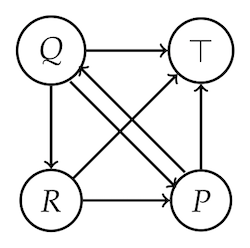
Updating our matrix $\A$ accordingly, we insert $\top$ in the first row/column: $$ \A = \left[ \begin{matrix} 0 & 1 & 1 & 1 \\
0 & 0 & 1 & 1 \\
0 & 1 & 0 & 0 \\
0 & 0 & 1 & 0 \end{matrix} \right]. $$ Redoing our limit anlaysis gives us the vector $(1.00, 0.57, 0.43, 0.33)$. But this isn’t our final answer, because it’s actually not possible for the non-$\top$ nodes to get a value higher than $2/3$ in a graph with just $3$ non-$\top$ nodes.⁴ So we divide elementwise by $(1, 2/3, 2/3, 2/3)$ to scale things, giving us our final result: $$ \left[ \begin{matrix} 1.00 \\
0.85 \\
0.65 \\
0.49 \end{matrix} \right]. $$ The relative justifications are the same as before, e.g. $P$ is still $1.3$ times as justified as $Q$. But now we can make absolute assessments too. $R$ comes out looking pretty bad ($0.49$), as seems right, while $Q$ looks a bit better ($0.65$). Of course $P$ looks best ($0.85$), though maybe not quite good enough to be justified tout court.

The Klein–Warfield Problem

Ok that’s theoretically nifty and all, but does it work on actual cases? Let’s try it out by looking at a notorious objection to coherentism. Klein & Warfield (1994) argue that coherentism flouts the laws of probability. How so?

Making sense of things often means believing more: taking on new beliefs to resolve the tensions in our existing ones. For example, if we think Tweety is a bird who can’t fly, the tension is resolved if we also believe they’re a penguin.⁵

But believing more means believing less probably. Increases in logical strength bring decreases in probability (unless the stronger content was already guaranteed with probability $1$). So increasing the coherence in one’s web of belief will generally mean decreasing its probability. How could increasing coherence increase justification, then?

Merricks (1995) points out that, even though the probability of the whole corpus goes down, the probabilities of individual beliefs go up in a way. After all, it’s more likely Tweety can’t fly if they’re a penguin, than if they’re just a bird of some unknown species.

That’s only the beginning of a satisfactory answer though. After all, we might not be justified in believing Tweety’s a penguin in the first place! Adding a new belief to support an existing belief doesn’t help if the new belief has no support itself. We need a more global assessment, which is where the present account shines.

Suppose we add $P$ = Tweety is a penguin to the network containing $B$ = Tweety is a bird and $\neg F$ = Tweety can’t fly. Will this increase the centrality/justification of $B$ and of $\neg F$? Yes, but we need to sort out the support relations to verify this.

Presumably $P$ supports $B$, and $\neg F$ too. But what about the other way around? If Tweety is a flightless bird, there’s a decent chance they’re a penguin. But it’s hardly certain; they might be an emu or kiwi instead. Come to think of it, isn’t support a matter of degree, so don’t we need finer tools than just on/off arrows?

Yes, and the refinement is easy. We accommodate degrees of support by attaching weights to our arrows. Instead of just placing a $1$ in our matrix $\A$ wherever the column-node points to the row-node, we put a number from the $[0,1]$ interval that reflects the strength of support. The same limit analysis as before still works, as it turns out. We just think of our inferential links as “leaky pipes” now, where weaker links make for leakier pipelines.

We still need concrete numbers to analyze the Tweety example. But it’s a toy example, so let’s just make up some plausible-ish numbers to get us going. Let’s suppose $1\%$ of birds are flightless, and birds are an even smaller percentage of the flightless things, say $0.1\%$. Let’s also pretend that $20\%$ of flightless birds are penguins.

Before believing Tweety is a penguin then, our web of belief looks like this:

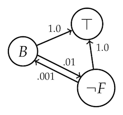
Calculating the degrees of justification for $B$ and $\neg F$, both come out very close to $0$ as you’d expect (with $B$ closer to $0$ than $\neg F$). Now we add $P$.

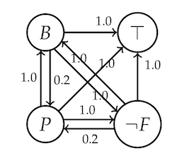
Recalculating degrees of justification, we find that they increase drastically. $B$ and $F$ are now justified to degree $0.85$, while $P$ is justified to degree $0.26$. (All numbers approximate.)

So our account vindicates Merricks. Not only does adding $P$ to the corpus add “local” justification for $B$ and for $\neg F$. It also improves their standing on a more global assessment.

You might be worried though: did $P$ come out too weakly justified, at just $0.26$? No: that’s either an artifact of oversimplification, or else it’s actually the appropriate outcome. Notice that $B$ and $\neg F$ don’t really support Tweety being a penguin. They’re a flightless bird, sure, but maybe they’re an emu, kiwi, or moa. We chose to believe penguin, and maybe we have our reasons. If we do, then the graph is missing background beliefs which would improve $P$’s standing once added. But otherwise, we just fell prey to stereotyping or comes-to-mind-bias, in which case it’s right that $P$ stand poorly.

Technical Background

The notion of centrality used here is a common tool in network analysis, where it’s known as “eigenvector centrality.” Because the frequency vector we arrive at in the limit is an eigenvector of the matrix $\A$. In fact it’s a special eigenvector, the only one with all-positive values.

Since we’re measuring justification on a $0$-to-$1$ scale, our account depends on there always being such an eigenvector for $\A$. In fact we need it to be unique, up to scaling (i.e. up to multiplication by a constant).

The theorem that guarantees this is actually quite old, going back to work by Oskar Perron and Georg Frobenius published around 1910. Here’s one version of it.

Perron–Frobenius Theorem. Let $\A$ be a square matrix whose entries are all positive. Then all of the following hold.

1. $\A$ has an eigenvalue $\lambda$ that is larger (in absolute value) than $\A$’s other eigenvalues. We call $\lambda$ the leading eigenvalue.
2. $\A$’s leading eigenvalue has an eigenvector $\v$ whose entries are all positive. We call $\v$ the leading eigenvector.
3. $\A$ has no other positive eigenvectors, save multiples of $\v$.
4. The powers $(\A/\lambda)^n$ as $n \rightarrow \infty$ approach a matrix whose columns are all multiples of $\v$.

Now, our matrices had some zeros, so they weren’t positive in all their entries. But it doesn’t really matter, as it turns out.

Frobenius’ contribution was to generalize this result to many cases that feature zeros. But even in cases where Frobenius’ weaker conditions aren’t satisfied, we can just borrow a trick from Google.⁶ Instead of using a $0$-to-$1$ scale, we use $\epsilon$-to-$1$ for some very small positive number $\epsilon$. Then all entries in $\A$ are guaranteed to be positive, and we just rescale our results accordingly. (Choose $\epsilon$ small enough and the difference is negligible in practice.)

Acknowledgments

This post owes a lot to prior work by Elena Derksen and Selim Berker. I’d never really thought much about how coherence and justification relate prior to reading Derksen’s work. And Berker’s prompted me to take graphs more seriously as a way of formalizing coherentism. I’m also grateful to David Wallace for introducing me to the Perron–Frobenius theorem’s use as a tool in network analysis.