This post is coauthored with Johanna Thoma and cross-posted at Choice & Inference. Accompanying Mathematica code is available on GitHub.

Lara Buchak’s Risk & Rationality advertises REU theory as able to recover the modal preferences in the Allais paradox. In our commentary we challenged this claim. We pointed out that REU theory is strictly “grand-world”, and in the grand-world setting it actually struggles with the Allais preferences.

To demonstrate, we constructed a grand-world model of the Allais problem. We replaced each small-world outcome with a normal distribution whose mean matches its utility, and whose height corresponds to its probability.

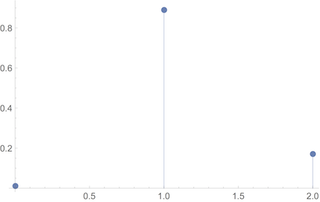
Take for example the Allais gamble: $$(\$0, .01; \$1M, .89; \$5M, .1).$$ If we adopt Risk & Rationality’s utility assignments: $$u(\$0) = 0, u(\$1M) = 1, u(\$5M) = 2,$$ we can depict the small-world version of this gamble:

On our grand-world model this becomes:

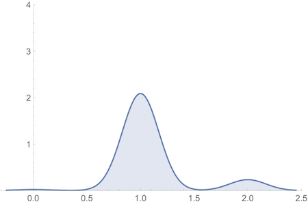
And REU theory fails to predict the usual Allais preferences on this model, provided the normal distributions used are minimally spread out.

If we squeeze the normal distributions tight enough, the grand-world problem collapses into the small-world problem, and REU theory can recover the Allais preferences. But, we showed, they’d have to be squeezed absurdly tight. A small standard deviation like $\sigma = .1$ lets REU theory recover the Allais preferences.¹ But it also requires outlandish certainty that a windfall of $\$$1M will lead to a better life than the one you’d expect to lead without it. The probability of a life of utility at most 0, despite winning $\$$1M, would have to be smaller than $1 \times 10^{-23}$.² Yet the chances are massively greater than that of suffering life-ruining tragedy (illness, financial ruin… Game of Thrones ending happily ever after, etc.).

In response Buchak offers two replies. The first is a technical maneuver, adjusting the model parameters. The second is more philosophical, adjusting the target interpretation of the Allais paradox instead.

First Reply

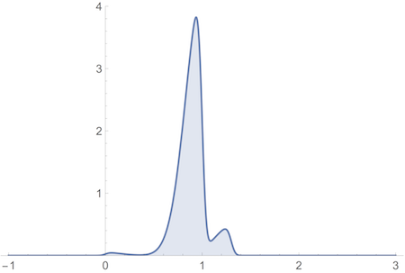
Buchak’s first reply tweaks our model in two ways. First, the mean utility of winning $\$$5M is shifted from 2 down to 1.3. Second, all normal distributions are skewed by a factor of 5 (positive 5 for utility 0, negative otherwise). So, for example, the Allais gamble pictured above becomes:

We’ll focus on the second tweak here, the introduction of skew. It rests on a technical error, as we’ll show momentarily. But it also wants for motivation.

Motivational Problems

Why should the grand-world model be skewed? And why in this particular way? Buchak writes:

[…] receiving $\$$1M makes the worst possibilities much less likely. Receiving $\$$1M provides security in the sense of making the probability associated with lower utility values smaller and smaller. The utility of $\$$1M is concentrated around a high mean with a long tail to the left: things likely will be great, though there is some small and diminishing chance they will be fine but not great. Similarly, the utility of $\$$0 is concentrated around a low mean with a long tail to the right: things likely will be fine but not great, though there is some small and diminishing chance they will be great. In other words, $\$$1M (and $\$$5M) is a gamble with negative skew, and $\$$0 is a gamble with positive skew …

But this passage never actually identifies any asymmetry in the phenomena we’re modeling. True, “receiving $\$$1M makes the worst possibilities much less likely”, but it also makes the best possibilities much more likely. Likewise, “[r]eceiving $\$$1M provides security in the sense of making the probability associated with lower utility values smaller and smaller.” But $\$$1M also makes the probability associated with higher utility values larger. And so on.

The tendencies of large winnings to control bad outcomes and promote good outcomes was already captured in the original model. A normal distribution centered on utility 1 already admits “some small and diminishing chance that [things] will be fine but not great.” It just also admits some small chance that things will be much better than great, since it’s symmetric around utility 1. To motivate the skewed model, we’d need some reason to think this symmetry should not hold. But none has been given.

Technical Difficulties

Motivation aside, there is a technical fault in the skewed model.

Introducing skew is supposed to make room for a reasonably large standard deviation while still recovering the Allais preferences. Buchak advertises a standard deviation³ of $\sigma = .17$ for the skewed model, but the true value is actually $.106$—essentially the same as the $.1$ value Buchak concedes is implausibly small, and seeks to avoid by introducing skew.⁴

Where does the $.17$ figure come from then? It’s the scale parameter of the skew normal distribution, often denoted $\omega$. For an ordinary normal distribution, the scale $\omega$ famously coincides with the standard deviation $\sigma$, and so we write $\sigma$ for both. But when we skew a normal distribution, we tighten it, shrinking the standard deviation:

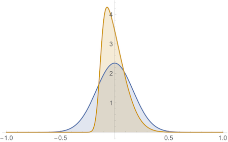
The distributions in this figure share the same scale parameter ($.17$) but the skewed one (yellow) is much narrower.⁵

Unfortunately, Mathematica uses $\sigma$ for the scale parameter even in skewed normal distributions, giving the misleading impression that it’s still the standard deviation.

What really matters, of course, isn’t the value of the standard deviation itself, but the probabilities that result from whatever parameters we choose. And Buchak argues that her model avoids the implausible probabilities we cited in the introduction. How can this be?

Buchak says that the skewed model has “more overlap in the utility that $\$$0 and $\$$1M might deliver”:

[…] there is a 0.003 probability that the $\$$0 gamble will deliver more than 0.5 utils, and a 0.003 probability that the $\$$1M gamble will deliver less than 0.5 utils. (p. 2402)

But this “overlap” was never the problematic quantity. The problem was, rather, that a small standard deviation like $.1$ requires you to think it less than $1 \times 10^{-23}$ likely you will end up with a life no better than $0$ utils, despite a $\$$1M windfall.

On Buchak’s model this probability is still absurdly small: $4 \times 10^{-9}$.⁶ This is a considerable improvement over $1 \times 10^{-23}$, but it’s still not plausible. For example, it’s almost $300,000$ times more likely that one author of this post (Jonathan Weisberg) will die in the coming year at the ripe old age of 39.

But worst of all, any improvement here comes at an impossible price: ludicrously low probabilities on the other side. For example, the probability that the life you’ll lead with $\$$1M will end up as good as the one you’d expect with $\$$5M is so small that Mathematica can’t distinguish it from zero.⁷ So the problem is actually worse than before, not better.

Second Reply

Buchak’s second reply is that it wouldn’t in fact be a problem if REU theory could only recover the Allais preferences in a small-world setting. We should think of the Allais problem as a thought experiment: it asks us to abstract away from anything but the immediate rewards mentioned in the problem, and to think of the monetary rewards as stand-ins for things that are valuable for their own sakes.

What Risk & Rationality showed, according to Buchak, is that REU theory can accommodate people’s intuitions regarding such a small-world thought experiment. And this is a success, because this establishes that the theory can accommodate a certain kind of reasoning that we all engage in. Buchak moreover concedes that it may well be a mistake for agents to think of the choices they actually face in small-world terms. But she claims this is no problem for her theory:

[I]f people ‘really’ face the simple choices, then their reasoning is correct and REU captures it. If people ‘really’ face the complex choices, then the reasoning in favor of their preferences is misapplied, and REU does not capture their preferences. Either way, the point still stands: REU-maximization rationalizes and formally reconstructs a certain kind of intuitive reasoning, as seen through REU theory’s ability to capture preferences over highly idealized gambles to which this reasoning is relevant. (p. 2403)

But there isn’t actually an ‘if’ here. People do really face ‘complex’ choices as we tried to model them. Any reward from an isolated gamble an agent faces in her life really should itself be thought of as a gamble. This is not only true when the potential reward is something like money, which is only a means to something else. Even if the good in question is ‘ultimate’, it just adds to the larger gamble of the agent’s life she is yet to face. She might win a beautiful holiday, but she will still face 20 micromorts per day for the rest of her life (24 if she moves from Canada to England). Even on our deathbeds, we are unsure about how a lot of things we care about will play out. REU theory makes this background risk relevant to the evaluation of any individual gamble.

So Buchak’s response really comes to this: REU theory captures a kind of intuitive reasoning that we employ in highly idealized decision contexts, but which would be misapplied in any actual decisions agents face in their lives. This raises two questions:

1. Why should we care about accommodating reasoning in highly idealized decision contexts?

   The original project of Risk & Rationality was to rationally accommodate the ordinary decision-maker. But now what we are rationally accommodating are at best her responses to thought experiments that are very far removed from her real life, namely thought experiments that ask her to imagine that she faces no other risk in her life. If our model is right, then REU theory still has to declare her irrational if she acts in real life as she would in the thought experiment—as presumably ordinary decision-makers do. And then we haven’t done very much to rationally accommodate her. At best, we have provided an error theory to explain her ordinary behaviour: her mistake is to treat grand-world problems like small-world problems. This is, of course, a different project than the one Risk & Rationality originally embarked on. As an error theory, REU theory will have to compete with other theories of choice under uncertainty that were never meant to be theories of rationality, such as prospect theory. Moreover, there is still another open question.

2. Why should agents have developed a knack for the reasoning displayed in the Allais problem if it is never actually rational to use it?

   As a heuristic to try and approximate the behaviour of a perfectly rational system, at least in the Allais example, agents would do better to maximize expected utility—which is also easier to compute. Moreover, the burden of proof is on proponents of REU theory to show that there are any grand-world decisions commonly faced by real agents where REU theory comes to a significantly different assessment than expected utility theory. Unless they can show this, expected utility theory comes out as the better heuristic more generally. It is then quite mysterious what explains our supposed employment of REU-style reasoning. Why should irrational agents, who employ it more generally, have developed a bad heuristic? And why should rational agents, who never use it in real life, develop a tendency to employ it exclusively in highly idealized thought experiments?

Ultimately, if Buchak’s first reply fails, and all we can rely on is her second reply, Risk & Rationality provides us with no reason to abandon expected utility theory as our best theory of rational choice under uncertainty in actual choice scenarios. Even if we grant that REU theory is a better theory of rational choice in hypothetical scenarios we never face, this is a much less exciting result than the one Risk & Rationality advertised.