In this and the next two posts we’ll establish the central theorem of the accuracy framework. We’ll show that the laws of probability are specially suited to the pursuit of accuracy, measured in Brier distance.

We showed this for cases with two possible outcomes, like a coin toss, way back in the first post of this series. A simple, two-dimensional diagram was all we really needed for that argument. To see how the same idea extends to any number of dimensions, we need to generalize the key ingredients of that reasoning to $n$ dimensions.

This post supplies the first ingredient: the convexity theorem.

Convex Shapes

Convex shapes are central to the accuracy framework because, in a way, the laws of probability have a convex shape. Hopefully that mystical pronouncement will make sense by the end of this post.

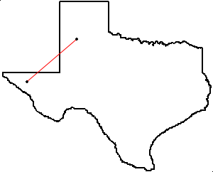
You probably know a convex shape when you see one. Circles, triangles, and octagons are convex; pentagrams and the state of Texas are not.

But what makes a convex shape convex? Roughly: it contains all its connecting lines. If you take any two points in a convex region and draw a line connecting them, the line will lie entirely inside that region.

But on a non-convex figure, you can find points whose connecting line leaves the figure’s boundary:

We want to take this idea beyond two dimensions, though. And for that, we need to generalize the idea of connecting lines. We need the concept of a “mixture”.

Pointy Arithmetic

In two dimensions it’s pretty easy to see that if you take some percentage of one point, and a complementary percentage of another point, you get a third point on the line between them.$ \renewcommand{\vec}[1]{\mathbf{#1}} \newcommand{\p}{\vec{p}} \newcommand{\q}{\vec{q}} \newcommand{\r}{\vec{r}} \newcommand{\v}{\vec{v}} \newcommand{\R}{\mathbb{R}} $

For example, if you take $1/ 2$ of $(0,0)$ and add it to $1/ 2$ of $(1,1)$, you get the point halfway between: $(1/ 2,1/ 2)$. That’s pretty intuitive geometrically: 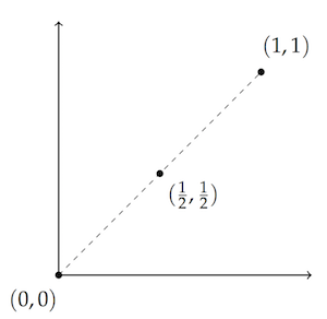But we can capture the idea algebraically too: $$ \begin{align} 1/ 2 \times (0,0) + 1/ 2 \times (1,1) &= (0,0) + (1/ 2, 1/ 2)\\
&= (1/ 2, 1/ 2). \end{align} $$

Likewise, if you add $3/10$ of $(0,0)$ to $7/10$ of $(1, 1)$, you get the point seven-tenths of the way in between, namely $(7/10, 7/10)$: 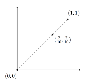In algebraic terms: $$ \begin{align} 3/10 \times (0,0) + 7/10 \times (1,1) &= (0,0) + (7/10, 7/10)\\
&= (7/10, 7/10). \end{align} $$

Notice that we just introduced two rules for doing arithmetic with points. When multiplying a point $\p = (p_1, p_2)$ by a number $a$, we get: $$ a \p = (a p_1, a p_2). $$ And when adding two points $\p = (p_1, p_2)$ and $\q = (q_1, q_2)$ together: $$ \p + \q = (p_1 + q_1, p_2 + q_2). $$ In other words, multiplying a point by a single number works element-wise, and so does adding two points together.

We can generalize these ideas straightforwardly to any number of dimensions $n$. Given points $\p = (p_1, p_2, \ldots, p_n)$ and $\q = (q_1, q_2, \ldots, q_n)$, we can define: $$ a \p = (a p_1, a p_2, \ldots, a p_n), $$ and $$ \p + \q = (p_1 + q_1, p_2 + q_2, \ldots, p_n + q_n).$$ We’ll talk more about arithmetic with points next time. For now, these two definitions will do.

Mixtures

Now back to connecting lines between points. The idea is that the straight line between $\p$ and $\q$ is the set of points we get by “mixing” some portion of $\p$ with some portion of $\q$.

We take some number $\lambda$ between $0$ and $1$, we multiply $\p$ by $\lambda$ and $\q$ by $1 - \lambda$, and we sum the results: $\lambda \p + (1-\lambda) \q$. The set of points you can obtain this way is the straight line between $\p$ and $\q$.

In fact, you can mix any number of points together. Given $m$ points $\q_1, \ldots, \q_m$, we can define their mixture as follows. Let $\lambda_1, \ldots \lambda_m$ be positive real numbers that sum to one. That is:

• $\lambda_i \geq 0$ for all $i$, and
• $\lambda_1 + \lambda_2 + \ldots + \lambda_m = 1$.

Then we multiply each $\q_i$ by the corresponding $\lambda_i$ and sum up: $$ \p = \lambda_1 \q_1 + \ldots + \lambda_m \q_m. $$ The resulting point $\p$ is a mixture of the $\q_i$’s.

Now we can define the general notion of a convex set of points. A convex set is one where the mixture of any points in the set is also contained in the set. (A convex set is “closed under mixing”, you might say.)

Convex Hulls

It turns out that the set of possible probability assignments is convex.

More than that, it’s the convex set generated by the possible truth-value assignments, in a certain way. It’s the “convex hull” of the possible truth-value assignments.

What in the world is a “convex hull”?

Imagine some points in the plane—the corners of a square, for example. Now imagine stretching a rubber band around those points and letting it snap tight. The shape you get is the square with those points as corners. And the set of points enclosed by the rubber band is a convex set. Take any two points inside the square, or on its boundary, and draw the straight line between them. The line will not leave the square.

Intuitively, the convex hull of a set of points in the plane is the set enclosed by the rubber band exercise. Formally, the convex hull of a set of points is the set of points that can be obtained from them as a mixture. (And this definition works in any number of dimensions.)

For example, any of the points in our square example can be obtained by taking a mixture of the vertices. Take the center of the square: it’s halfway between the bottom left and top right corners. To get something to the left of that we can mix in some of the top left corner (and correspondingly less of the top right). And so on.

Now imagine the rubber band exercise using the possible truth-value assignments, instead of the corners of a square. In two dimensions, those are the points $(0,1)$ and $(1,0)$. And when you let the band snap tight, you get the diagonal line connecting them. As we saw way back in our first post, the points on that diagonal line are the possible probability assignments.

Peeking Ahead

We also saw that if you take any point not on that diagonal, the closest point on the diagonal forms a right angle. That’s what lets us do some basic geometric reasoning to see that there’s a point on the line that’s closer to both vertices than the point off the line:

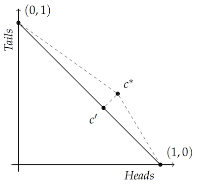
That fact about closest points and right angles is what’s going to enable us to generalize the argument beyond two dimensions. If you take any point not on a convex hull, there’s a point on the convex hull (namely the closest point) which forms a right (or obtuse) angle with the other points on the hull.

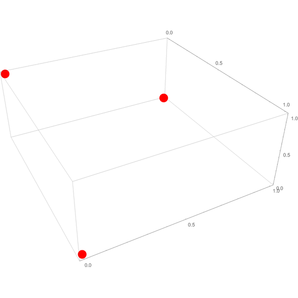
Consider the three dimensional case. The possible truth-value assignments are $(1,0,0)$, $(0,1,0)$, and $(0,0,1)$: And when you let a rubber band snap tight around them, it encloses the triangular surface connecting them: 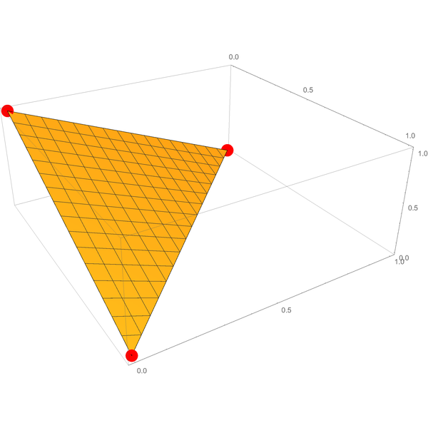That’s the set of probability assignments for three outcomes.

Now take any point that’s not on that triangular surface. Drop a straight line to the closest point on the surface. Then draw another straight line from there to one of the triangle’s vertices. These two straight lines will form a right or obtuse angle. So the distance from the first, off-hull point to the vertex is further than the distance from the second, on-hull point to the vertex.

Essentially the same reasoning works in any number of dimensions. But to make it work, we need to do three things.

1. Prove that the probability assignments always form a convex hull around the possible truth-value assignments.
2. Prove that any point outside a convex hull forms a right angle (or an obtuse angle) with any point on the hull.
3. Prove that the point off the hull is further from all the vertices than the closest point on the hull.

This post is dedicated to the first item.

The Convexity Theorem

We’re going to prove that the set of possible probability assignments is the same as the convex hull of the possible truth-value assignments. First let’s get some notation in place.

Notation

As usual $n$ is the number of possible outcomes under consideration. So each possible truth-value assignment is a point of $n$ coordinates, with a single $1$ and $0$ everywhere else. For example, if $n = 4$ then $(0, 0, 1, 0)$ represents the case where the third possibility obtains.

We’ll write $V$ for the set of all possible truth value assignments. And we’ll write $\v_1, \ldots, \v_n$ for the elements of $V$. The first element $\v_1$ has its $1$ in the first coordinate, $\v_2$ has its $1$ in the second coordinate, etc.

We’ll use a superscript $^+$ for the convex hull of a set. So $V^+$ is the convex hull of $V$. It’s the set of all points that can be obtained by mixing members of $V$.

Recall, a mixture is a point obtained by taking nonnegative real numbers $\lambda_1, \ldots, \lambda_n$ that sum to one, and multiplying each one against the corresponding $\v_i$ and then summing up: $$ \lambda_1 \v_1 + \lambda_2 \v_2 + \ldots + \lambda_n \v_n. $$ So $V^+$ is the set of all points that can be obtained by this method. Each choice of values $\lambda_1, \ldots, \lambda_n$ generates a member of $V^+$. (To exclude one of the $\v_i$’s from a mixture, just set $\lambda_i = 0$.)

Finally, we’ll use $P$ for the set of all probability assignments. Recall: a probability assignment is a point of $n$ coordinates, where each coordinate is nonnegative, and all the coordinates together add up to one. That is, $\p = (p_1,\ldots,p_n)$ is a probability assignment just in case:

• $p_i \geq 0$ for all $i$, and
• $p_1 + p_2 + \ldots + p_n = 1$.

The set $P$ contains just those points $\p$ satisfying these two conditions.

Statement and Proof

In the notation just established, what we’re trying to show is that $V^+ = P$.

Theorem. $V^+ = P$. That is, the convex hull of the possible truth-value assignments just is the set of possible probability assignments.

Proof. Let’s first show that $V^+ \subseteq P$.

Notice that a truth-value assignment is also probability assignment. Its coordinates are always $1$ or $0$, so all coordinates are nonnegative. And since it has only a single coordinate with value $1$, its coordinates add up to $1$.

But we have to show that any mixture of truth-value assignments is also a probability assignment. So let $\lambda_1, \ldots, \lambda_n$ be nonnegative numbers that sum to $1$. If we multiply $\lambda_i$ against a truth-value assignment $\v_i$, we get a point with $0$ in every coordinate except the $i$-th coordinate, which has value $\lambda_i$. For example, $\lambda_3 \times (0, 0, 1, 0) = (0, 0, \lambda_3, 0)$. So the mixture that results from $\lambda_1, \ldots, \lambda_n$ is: $$ \lambda_1 \v_1 + \lambda_2 \v_2 + \ldots \lambda_n \v_n = (\lambda_1, \lambda_2, \ldots, \lambda_n). $$ And this mixture has coordinates that are all nonnegative and sum to $1$, by hypothesis. In other words, it is a probability assignment.

So we turn to showing that $P \subseteq V^+$. In other words, we want to show that every probability assignment can be obtained as a mixture of the $\v_i$’s.

So take an arbitrary probability assignment $\p \in P$, where $\p = (p_1, \ldots, p_n)$. Let the $\lambda_i$’s be the probabilities that $\p$ assigns to each $i$: $\lambda_1 = p_1$, $\lambda_2 = p_2$, and so on. Then, by the same logic as in the first part of the proof: $$ \lambda_1 \v_1 + \ldots + \lambda_n \v_n = (p_1, \ldots, p_n). $$ In other words, $\p$ is a mixture of the possible truth-value assignments, where the weights in the mixture are just the probability values assigned by $\p$. $\Box$

Up Next

We’ve established the first of the three items listed earlier. Next time we’ll establish the second: given a point outside a convex set, there’s always a point inside that forms a right or obtuse angle with any other point of the set. Then we’ll be just a few lines of algebra from the main result: the Brier dominance theorem!