Last time we saw why accuracy-mavens prefer Brier distance to Euclidean distance. But we did everything in two dimensions. That’s fine for a coin toss, with only two possibilities. But what if there are three doors and one of them has a prize behind it??

Don’t panic! Today we’re going to verify that Brier distance is still a proper way of measuring inaccuracy, even when there are more than two possibilities. (Next time we’ll talk about Euclidean distance with more than two possibilitie.)

Let’s start small, with just three possibilities. $\renewcommand{\vec}[1]{\mathbf{#1}}\newcommand{\p}{\vec{p}}\newcommand{\q}{\vec{q}}\newcommand{\v}{\vec{v}}\newcommand{\EIpq}{EI_{\p}(\q)}\newcommand{\EIpp}{EI_{\p}(\p)}$

Three Possibilities

You’re on a game show; there are three doors; one has a prize behind it. The three possibilities are represented by the vertices $(1,0,0)$, $(0,1,0)$, and $(0,0,1)$:

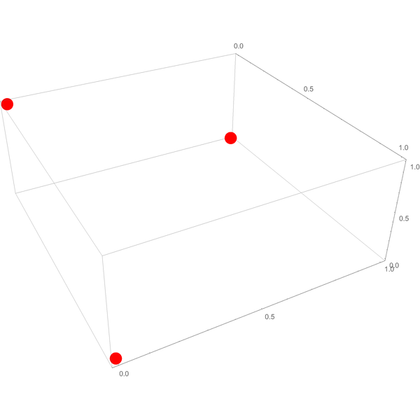
Your credences are given by some probability assignment $(p_1, p_2, p_3)$. It might be $(1/ 3, 1/ 3, 1/ 3)$ but it could be anything… $(7/ 10, 2/ 10, 1/ 10)$, for example.

In case you’re curious, here’s what the range of possible probability assignments looks like in graphical terms:

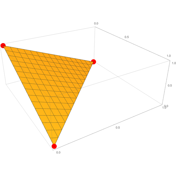
The triangular surface is the three-dimensional analogue of the diagonal line in the two-dimensional diagram from our first post in this series.

It’ll be handy to refer to points on this surface using single letters, like $\p$ for $(p_1, p_2, p_3)$. We’ll write these letters in bold, to distinguish a sequence of numbers like $\p$ from a single number like $p_1$. (In math-speak, $\p$ is a vector and $p_1$ is a scalar.)

Our job is to show that Brier distance is “proper” in three dimensions. Let’s recall what that means: given a point $\p$, the expected Brier distance (according to $\p$) of a point $\q = (q_1, q_2, q_3)$ from the three vertices is always smallest when $\q = \p$.

What does that mean?

Recall, the Brier distance from $\q$ to the vertex $(1, 0, 0)$ is: $$ (q_1 - 1)^2 + (q_2 - 0)^2 + (q_3 - 0)^2 $$ Or, more succinctly: $$ (q_1 - 1)^2 + q_2^2 + q_3^2 $$ So the expected Brier distance of $\q$ according to $\p$ weights each such sum by the probability $\p$ assigns to the corresponding vertex. $$ \begin{align} &\quad\quad p_1 \left( (q_1 - 1)^2 + q_2^2 + q_3^2 \right)\\
&\quad + p_2 \left( q_1^2 + (q_2 - 1)^2 + q_3^2 \right)\\
&\quad + p_3 \left( q_1^2 + q_2^2 + (q_3 - 1)^2 \right) \end{align} $$ We need to show that this quantity is smallest when $\q = \p$, i.e. when $q_1 = p_1$, $q_2 = p_2$, and $q_3 = p_3$.

Visualizing Expected Inaccuracy

Let’s do some visualization. We’ll take a few examples of $\p$, and graph the expected inaccuracy of other possible points $\q$, using Brier distance to measure inaccuracy.

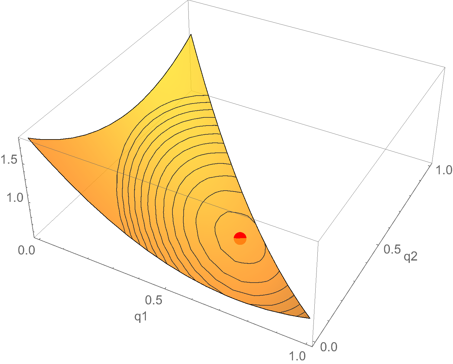
For example, suppose $\p = (1/ 3, 1/ 3, 1/ 3)$. Then the expected inaccuracy of each point $\q$ looks like this:

The horizontal axes represent $q_1$ and $q_2$. The vertical axis represents expected inaccuracy.

Where’s $q_3$?? Not pictured! If we used all three visible dimensions for the elements of $\q$, we’d have nothing left to visualize expected inaccuracy. But $q_3$ is there implicitly. You can always get $q_3$ by calculating $1 - (q_1 + q_2)$, because $\q$ is a probability assignment. So we don’t actually need $q_3$ in the graph!

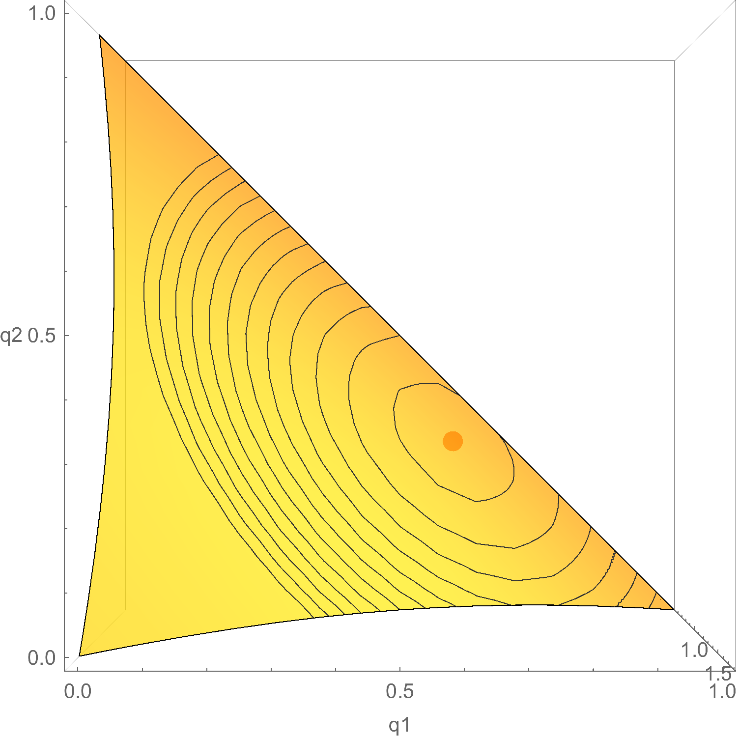
Now, the red dot is the lowest point on the surface: the smallest possible expected inaccuracy, according to $\p$. But where is that in terms of $q_1$ and $q_2$? Let’s look at the same graph from directly above:

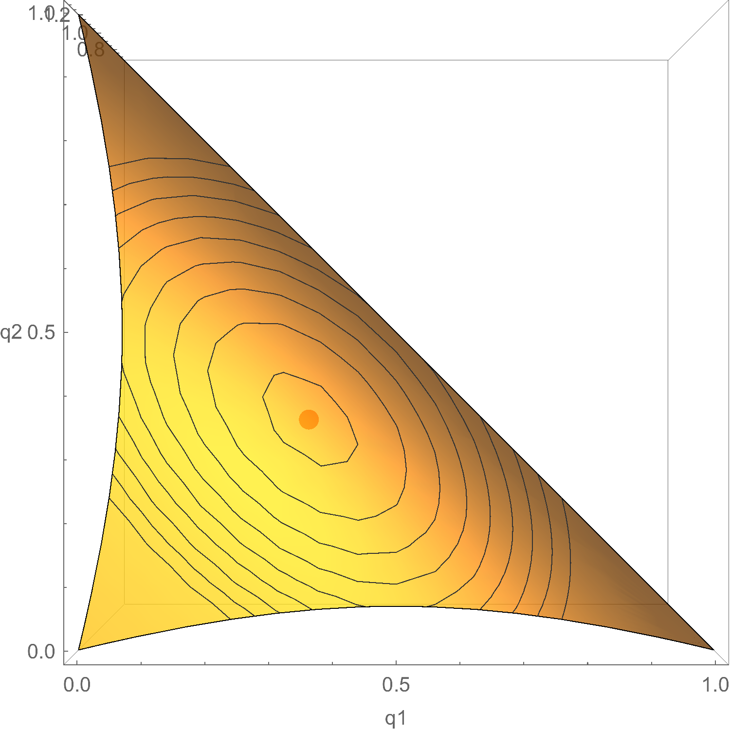
Hey! Looks like the red dot is located at $q_1 = 1/ 3$ and $q_2 = 1/ 3$, i.e. at $\q = (1/ 3, 1/ 3, 1/ 3)$. Also known as $\p$. So that’s promising: looks like expected inaccuracy is minimized when $\q = \p$, at least in this example.

Let’s do one more example, $\p = (6/ 10, 3/ 10, 1/ 10)$. Then the expected Brier distance of each point $\q$ looks like this: Or, taking the aerial view again: Yep, looks like the red dot is located at $q_1 = 6/ 10$ and $q_2 = 3/ 10$, i.e. at $\q = (6/ 10, 3/ 10, 1/ 10)$, also known as $\p$. So, once again, it seems expected inaccuracy is minimized when $\q = \p$.

So let’s prove that that’s how it always is.

A Proof

We’ll need a little notation: I’m going to write $\EIpq$ for the expected inaccuracy of point $\q$, according to $\p$.

Now recall our formula for expected inaccuracy: $$ \begin{align} \EIpq &= \quad p_1 \left( (q_1 - 1)^2 + q_2^2 + q_3^2 \right)\\
&\quad + p_2 \left( q_1^2 + (q_2 - 1)^2 + q_3^2 \right)\\
&\quad + p_3 \left( q_1^2 + q_2^2 + (q_3 - 1)^2 \right). \end{align} $$ How do we find the point $\q$ that minimizes this mess?

Originally this post used some pretty tedious calculus. But thanks to a hot tip from Jonathan Love, we can get by just with algebra.

First we need to expand the squares in our big ugly sum: $$ \begin{align} \EIpq &= \quad p_1 \left( q_1^2 - 2q_1 + 1 + q_2^2 + q_3^2 \right)\\
&\quad + p_2 \left( q_1^2 + q_2^2 - 2q_2 + 1 + q_3^2 \right)\\
&\quad + p_3 \left( q_1^2 + q_2^2 + q_3^2 - 2q_3 + 1 \right). \end{align} $$ Then we’ll gather some common terms and rearrange things: $$ \begin{align} \EIpq &= (p_1 + p_2 + p_3)\left(q_1^2 + q_2^2 + q_3^2 + 1 \right) - 2p_1q_1 - 2p_2q_2 - 2p_3q_3.\\
\end{align} $$ Since $p_1 + p_2 + p_3 = 1$, that simplifies to: $$ \begin{align} \EIpq &= q_1^2 + q_2^2 + q_3^2 + 1 - 2p_1q_1 - 2p_2q_2 - 2p_3q_3.\\
\end{align} $$

Now we’ll use Jonathan’s ingenious trick. We’re going to add $p_1^2 + p_2^2 + p_3^2 - 1$ to this expression, which doesn’t change where the minimum occurs. If you shift every point on a graph upwards by the same amount, the minimum is still in the same place. (Imagine everybody in the world grows by an inch overnight; the shortest person in the world is still the shortest, despite being an inch taller.)

Then, magically, we get an expression that factors into something tidy: $$ \begin{align} &\phantom{=}\phantom{=} p_1^2 + p_2^2 + p_3^2 + q_1^2 + q_2^2 + q_3^2 - 2p_1q_1 - 2p_2q_2 - 2p_3q_3\\
&= (p_1 - q_1)^2 + (p_2 - q_2)^2 + (p_3 - q_3)^2. \end{align} $$ And not just tidy, but easy to minimize. It’s a sum of squares, and squares are never negative. So the smallest possible value is $0$, which occurs when all the squares are $0$, i.e. when $q_1 = p_1$, $q_2 = p_2$, and $q_3 = p_3$.

So, the minimum of $\EIpq$ occurs in the same place, namely when $\q = \p$!

The Nth Dimension

Now we can use the same idea to generalize to any number of dimensions. Since the steps are essentially identical, I’ll keep it short and (I hope) sweet.

Theorem.  Given a probability assignment $\p = (p_1, \ldots, p_n)$, if inaccuracy is measured using Brier distance, then $\EIpq$ is uniquely minimized when $\q = \p$.

Proof.  Let $\p = (p_1, \ldots, p_n)$ be a probability assignment, and let $\EIpq$ be the expected inaccuracy according to $\p$ of probability assignment $\q = (q_1, \ldots, q_n)$, measured using Brier distance.

First we simplify our expression for $\EIpq$ using algebra: $$ \begin{align} \EIpq &= \quad p_1 \left( (q_1 - 1)^2 + q_2^2 + \ldots + q_n^2 \right)\\
&\quad + p_2 \left( q_1^2 + (q_2 - 1)^2 + \ldots + q_n^2 \right)\\
&\quad\quad \vdots\\
&\quad + p_n \left( q_1^2 + q_2^2 + \ldots + q_{n-1}^2 + (q_n - 1)^2 \right)\\
&= (p_1 + \ldots + p_n)\left( q_1^2 + \ldots + q_n^2 + 1\right) - 2 p_1 q_1 - \ldots - 2 p_n q_n\\
&= q_1^2 + \ldots + q_n^2 + 1 - 2 p_1 q_1 - \ldots - 2 p_n q_n. \end{align} $$ Now, because $p_1^2 + \ldots + p_n^2 - 1$ is a constant, adding it to $\EIpq$ doesn’t change where the minimum occurs. So we can minimize instead: $$ \begin{align} &\phantom{=}\phantom{=} p_1^2 + \ldots + p_n^2 + q_1^2 + \ldots + q_n^2 - 2 p_1 q_1 - \ldots - 2 p_n q_n\\
&= (p_1 - q_1)^2 + \ldots + (p_n - q_n)^2. \end{align} $$ Being a sum of squares, the minimum value here cannot be less than $0$, which occurs when $\q = \p$. $\Box$

Conclusion

So what did we learn? That Brier distance isn’t just “stable” in toy cases like a coin-toss. It’s also stable in toy cases with any finite number of outcomes.

No matter how many outcomes are under consideration, each probability assignment expects itself to do best at minimizing inaccuracy, if we use Brier distance to measure inaccuracy.

To go beyond toy cases, we’d have to extend this result to cases with infinite numbers of possibilities. And I haven’t even begun to think about how to do that.

Instead, next time we’ll look at what happens in $3+$ dimensions when we use Euclidean distance instead of Brier distance. And it’s actually kind of interesting! It turns out Euclidean distance is still improper in $3+$ dimensions, but not necessarily in the same way as in $2$ dimensions. More on that next time…