If you’ve bumped into the accuracy framework before, you’ve probably seen a diagram like this one:
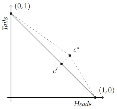
The vertices $(1,0)$ and $(0,1)$ represent two possibilities, whether a coin lands heads or tails in this example.
According to the laws of probability, the probability of heads and of tails must add up to $1$, like $.3 + .7$ or $.5 + .5$. So the diagonal line connecting the two vertices covers all the possible probability assignments… $(0,1)$, $(.3,.7)$, $(.5, .5)$, $(.9, .1)$, $(1,0)$, etc.$\newcommand{\vone}{(1,0)}$$\newcommand{\vtwo}{(0,1)}$
The diagram illustrates a key fact of the accuracy framework. Assignments that obey the laws of probability are always “closer to the truth” than assignments that violate those laws—no matter what the truth turns out to be. Given any point not on the line, there is a point on the line that is closer to both vertices $\vone$ and $\vtwo$. So, whether the coin lands heads or tails, you’ll be closer to the truth if your degrees of belief (a.k.a. “credences”) obey the laws of probability.
Take $c^*$, for example, which doesn’t lie on the diagonal line. Let’s assume $c^*$ is the point $(.7, .5)$, which violates the laws of probability: $.7 + .5 > 1$. Now compare that to $c’$, which does lie on the diagonal line. That’s the point $(.6, .4)$, which does obey the laws of probability: $.6 + .4 = 1$.
Well, $c’$ is closer to $\vone$ than $c^*$ is. Just look at the right-triangle connecting all three points: to get to $\vone$ from $c^*$ you have to travel along the hypotenuse. But you only have to travel the distance of one of the legs to get there from $c’$. And the same thinking applies to the other vertex, $\vtwo$. So $c’$ is closer to both vertices than $c^*$ is.
The same idea applies to any point in the unit square. If it’s not on the diagonal line, there’s a point on the line that will be closer to both vertices—because Pythagoras. Just go from whatever $c^*$ you start with to the closest point $c’$ on the diagonal. You’ll have two right-triangles, one for each vertex. So the $c’$ point will be closer to both vertices than the $c^*$ point you started with.
What’s more, no point on the line is closer to both vertices than any other. For example, if you move from $(.5, .5)$ to some other point on the line, you’ll move towards one vertex but away from the other. So if you’re off the line, you can always get closer to both vertices by moving onto the line. But once you’re on the line, there’s no way that guarantees you’ll be closer to the vertex representing the true outcome of the coin toss.
And that’s why you should obey the laws of probability, according to advocates of the accuracy framework. Violating the laws of probability takes you away from the truth, no matter what the truth turns out to be. Whereas if you obey the laws of probability, that doesn’t happen.
Hey, Dummy
If you’re like me, the first time you see this argument you think to yourself: “Cool! The diagram gives me the key idea, I’ll worry about mathematical technicalities later (like, what if there are more than two possibilities?). For now let me just see where you’re going with this, epistemology-wise…”
But when I finally did sit down to work through the math, I found it much harder than I expected to answer some elementary questions. The answers to these questions were usually taken for granted in published work, or they went by so fast I wasn’t sure about the details.
I’m still working on filling in a lot of these gaps, as I work through Richard Pettigrew’s excellent new book and get up to speed (I hope!) with the latest research. I’m writing these posts to help me get clear on the basics, and hopefully help you do the same.

(Warning: since I’m learning this stuff as I go, my solutions and proofs won’t always be the best. In fact they’re bound to have errors. So I encourage you to contact me with corrections, and help improve these posts for others.)
Now on to today’s topic: Euclidean distance as a measure of accuracy.
Fear of a Euclidean Plane
We just saw that the laws of probability keep you close to the truth in our coin-toss example, whatever the truth turns out to be. And by “close” we meant Euclidean distance, the kind of spatial distance familiar from grade-school geometry.
But people writing in the accuracy framework never use Euclidean distance. Why not? Because, it turns out, Euclidean distance is unstable!
“Unstable” how?
Well, if your aim is to be as close to the truth as possible in terms of Euclidean distance, then you will almost always be driven to change your opinion to something extreme: either $(1,0)$ or $(0,1)$. And not because you get some definite information about how the coin-flip turns out. But just because of the way Euclidean distance interacts with expected value. (I’m going to assume you’re familiar with the notion of expected value. If not, you can read the linked section of the SEP article or do a bit of googling.)
Here’s how that happens. Suppose your credences in heads/tails are $(.6, .4)$: you’re $60\%$ confident the coin will land heads, and $40\%$ confident it’ll land tails. What’s your expected inaccuracy, then? If we think of accuracy as utility, and thus inaccuracy as disutility, how well can you expect to do by holding your current state of opinion?
Let’s run the calculation. We’ll write $EI(x, 1-x)$ for the expected inaccuracy of having credence $x$ in heads and $1-x$ in tails.
$$
\begin{align}
EI(.6, .4) &= .6 \sqrt{(.6 - 1)^2 + (.4 - 0)^2} + .4 \sqrt{(.6 - 0)^2 + (.4 - 1)^2}\\
&= .6 \sqrt{(-.4)^2 + .4^2} + .4 \sqrt{.6^2 + (-.6)^2}\\
&= .678823
\end{align}
$$
Ok, not bad. But now let’s compare that to how you can expect to do if you change your opinion to the extreme state $(1,0)$:
$$
\begin{align}
EI(1, 0) &= .6 \sqrt{(1 - 1)^2 + (0 - 0)^2} + .4 \sqrt{(1 - 0)^2 + (0 - 1)^2}\\
&= .565685
\end{align}
$$
Some things to keep in mind here:
- The numbers outside the square root symbols are $.6$ and $.4$ because those are your current beliefs, and we’re asking how well you expect to do according to your current beliefs.
- The numbers inside the square roots are $1$ and $0$ because we’re asking how well you expect to do by adopting those extreme opinions. So those numbers describe the outcomes whose inaccuracy we want to evaluate and weigh.
- Remember, smaller numbers are better because we’re talking about inaccuracy.
And look: the extreme opinion $(1, 0)$ does better than the more moderate opinion you actually hold, $(.6, .4)$. The extreme opinion has lower expected inaccuracy (think: higher expected accuracy).
In fact, the extreme assignment does better than the moderate one according to the moderate assignment itself. So your moderate opinions end up undermining themselves. They drive you to hold more extreme opinions than you initially do, in the name of accuracy.
This isn’t an artifact of the particular example $(.6, .4)$. We can prove that an extreme state of opinion always does best in terms of expected inaccuracy—unless you are completely uncertain about the outcome, i.e. $(.5,.5)$.
Theorem.
Suppose $p \in [0, 1]$ and $p \neq .5$. Then, according to the probability assignment $(p, 1-p)$, the expected Euclidean distance of any alternative assignment $(q, 1-q)$ from the points $(1,0)$ and $(0,1)$ is uniquely minimized by:
$$
q = \begin{cases}
0 & \mbox{ if } p < .5,\\
1 & \mbox{ if } p > .5.
\end{cases}
$$
Proof.
Suppose $0 \leq p \leq 1$ and $p \neq .5$. According to the probability assignment $(p, 1-p)$, the expected Euclidean distance from $(1,0)$ and $(0,1)$ of any alternative assignment $(q, 1-q)$ is:
$$
\begin{align}
EI(q, 1-q) &= p \sqrt{(q - 1)^2 + ((1-q) - 0)^2}\\
&\quad + (1-p) \sqrt{(q - 0)^2 + ((1-q) - 1)^2}\\
&= p \sqrt{(q - 1)^2 + (1 - q)^2} + (1-p) \sqrt{q^2 + q^2}\\
&= p \sqrt{2} (1 - q) + (1-p) \sqrt{2} q\\
&= \sqrt{2} \left( p (1 - q) + (1-p) q \right).
\end{align}
$$
We are looking for the value of $q$ that minimizes the quantity on the last line, which is the same if we drop the $\sqrt{2}$ and just seek to minimize:
$$ p (1 - q) + (1-p) q. $$
This quantity is a weighted average of the two values $p$ and $(1-p)$, with the weights being $1-q$ and $q$, respectively. So the minimum possible value is just whichever of $p$ or $1-p$ is smaller. And this minimum is achieved when all the weight is given to the smaller value.
So, if $p < .5$, then the minimum possible value is $p$, and it is achieved when $1 - q = 1$, and thus $q = 0$. If instead $p > .5$, the minimum possible value is $1 - p$ and is achieved when $q = 1$. $\Box$
Based on this proof you can also see what happens when $p=.5$. It doesn’t matter what value $q$ takes: any value $0 \leq q \leq 1$ will result in the same expected inaccuracy, namely $.5\sqrt{2}$.
So here’s the problem with Euclidean distance as a way of measuring inaccuracy. As soon as you find yourself leaning one way or another on heads-vs.-tails, you’re driven to extremes. If you get information that makes heads slightly more likely, say $.51$ for example, your expected inaccuracy is minimized by leaping to the conclusion that the coin will certainly come up heads.
So any probability assignment to heads/tails besides $(.5, .5)$ is self-undermining. It gives you cause to adopt some other assignment—an extreme one, at that.
Even at $(.5, .5)$ things aren’t so happy, btw. Any other assignment of probabilities is just as good as far as minimizing inaccuracy goes. So even if the pursuit of accuracy doesn’t require you to change your opinion, it still permits you to do so. As far as accuracy goes, being indifferent about the coin toss also makes you indifferent about what opinion to hold. Which is pretty strange in itself.
Where This Leaves Us
Wait a minute: if Euclidean distance is a bad way to measure inaccuracy, then what’s the use of the diagram we started with?? And what’s the right way to measure inaccuracy?
We’ll tackle these questions in the next post. But here’s the short answer.
One common way of measuring inaccuracy is a variation on Euclidean distance called Brier distance. Brier distance is just enough like Euclidean distance to vindicate the reasoning we did with our opening diagram. But it’s different enough from Euclidean distance to avoid the instability problem we ended up with.
So what is Brier distance? It’s just the square of Euclidean distance. Just take the square root symbol off Euclid’s formula and you’ve got the formula for Brier distance. Next time we’ll see how that one change makes all the right differences.