How much does a PhD from a prestigious program help you on the job market in academic philosophy?
It makes a big difference to where you get a tenure-track job, if you do get one (see here). It also seems to make some difference to whether you get a tenure-track job (though maybe not as much as one might have thought: see here).
But here I want to consider whether it makes a difference to how long it takes to get a tenure-track job, if you do get one.
A priori I would have guessed a prestigious PhD shortens one’s expected time on the job market. But in some correspondence about my last two posts, the oppposite hypothesis came up. The thought is that prestigious PhDs are more likely to make stopovers in postdocs and fellowships before arriving at the tenure track. But then, on the third hand, maybe less prestigious PhDs are actually more likely to make stopovers, just in less cushy temporary gigs.
So which is it: does PhD prestige shorten expected time to the tenure track, or lengthen it?
Curiously, the answer so far seems to be: neither. If we use PGR ratings to measure prestige, and data from the APDA homepage to measure time-to-TT, there seems to be almost no connection. (Again, that’s assuming you do end up in a tenure-track job, which a prestigious PhD does seem to help with at least a bit.)
Because this conclusion surprised me so much (and because it’s likely to be controversial, even weaponized in the PGR wars), I’m going to make this post way more pedantic than usual. I’m going to walk through the analysis one step at a time, and even show all the code.
Hopefully, this way, careful readers will catch and correct any errors. And non-careful readers will be so turned off they’ll shut up and go away (instead of @-ing me with their volcanic takes on twitter or stirring up shit elsewhere in the blogosphere).
Ok let’s get started.
Setting Up
As usual I’m working in R, and since I’m a Hadley
stan we start by importing the tidyverse package. But we’ll also
import the tools package for its toTitleCase function, so that we
can enforce consistent capitalization. We’ll be combining data from two
different sources, the PGR and the APDA, so we’ll need the names of PhD
programs capitalized the same way in order to join the two datasets
properly.
library(tidyverse)
library(tools)
Next we import the APDA data. This is the same data scraped from the APDA homepage in my last post:
df_apda <- read_csv("data/apda-2018-11-9.csv",
                    col_types = cols(
                      grad_program = col_character(),
                      id = col_character(),
                      year_graduated = col_character(),
                      aos = col_character(),
                      year = col_integer(),
                      placement_program = col_character(),
                      type = col_character()
                    ))
It needs a bit of cleaning: we standardize the capitalization, fix a few typos… but we also filter out duplicate entries, entries where the year of the placement is missing or unknown, and entries where the type (TT/postdoc/etc.) is missing:
df_apda$grad_program <- toTitleCase(df_apda$grad_program)

df_apda$year[df_apda$year == 19182] <- 1982
df_apda$year[df_apda$year == 2104] <- 2014

df_apda <- df_apda %>%
  distinct() %>%
  filter(!is.na(year)) %>%
  filter(year_graduated != "Current Student or Graduation Year Unknown") %>%
  filter(!is.na(type))

df_apda$year_graduated <- as.integer(df_apda$year_graduated)
Next we calculate time_to_tt as follows: (i) filter out all but TT
placements, (ii) select the first placement (by year) for each graduate,
and (iii) subtract the year they graduated from that:
df_apda <- df_apda %>%
  filter(type == "Tenure-Track") %>%
  group_by(grad_program, id) %>%
  arrange(year) %>%
  slice(1) %>%
  mutate(time_to_tt = year - year_graduated) %>%
  ungroup()
For a glimpse of the results, here are ten randomly chosen entries:
set.seed(42)
sample_n(df_apda, 10) %>%
  select(grad_program, year_graduated, year, time_to_tt)
## # A tibble: 10 x 4
##    grad_program                        year_graduated  year time_to_tt
##    <chr>                                        <int> <dbl>      <dbl>
##  1 University of Virginia                        2011  2014          3
##  2 University of Wisconsin-Madison               2013  2016          3
##  3 New York University                           2016  2015         -1
##  4 University of Pittsburgh                      2014  2014          0
##  5 University of Edinburgh                       2015  2017          2
##  6 University of California, Davis               2003  2009          6
##  7 University of Minnesota Twin Cities           2011  2015          4
##  8 Emory University                              2007  2007          0
##  9 University of Illinois at Chicago             1996  2005          9
## 10 University of Memphis                         2012  2014          2
Now we import the PGR data:
df_pgr <- read_csv("data/pgr/pgr.csv",
                   col_types = cols(program = col_character(),
                                    mean = col_double(),
                                    locale = col_character(),
                                    year = col_integer()))
A random glimpse again:
sample_n(df_pgr, 10)
## # A tibble: 10 x 4
##    program                             mean locale       year
##    <chr>                              <dbl> <chr>       <int>
##  1 University of British Columbia       3   Canada       2017
##  2 University of Missouri               2.2 US           2008
##  3 University of Wisconsin-Madison      3.2 US           2008
##  4 Ohio State University                3.1 US           2008
##  5 University of British Columbia       2.6 Canada       2011
##  6 York University                      1.8 Canada       2008
##  7 Washington University in St. Louis   3.3 US           2017
##  8 Florida State University             2.3 US           2014
##  9 University of Calgary                2.3 Canada       2017
## 10 University of Canterbury             1.5 Australasia  2008
Note that we have ratings from the last six iterations of the PGR here: 2006, 2008, 2009, 2011, 2014, 2017. So we can pair graduates with PGR ratings from around the time they went on the market.
More precisely, we’ll assign each graduate a pgr_year corresponding to
the latest report available the year they graduated. Unless they
graduated prior to 2006 in which case we just use the 2006 ratings:
pgr_years <- unique(df_pgr$year)
df_apda <- df_apda %>%
  group_by(grad_program, id) %>%
  mutate(pgr_year = ifelse(year_graduated <= 2006,
                           2006,
                           max(pgr_years[pgr_years <= year_graduated]))) %>%
  ungroup()
(Yes yes we could get earlier PGR data but frankly I’m too lazy to go through all that again. Most of our graduates are from 2006 or later anyway, virtually all are from 2000 or later, and PGR scores don’t change too much from iteration to iteration.)
Finally, we join our two tables together, matching by program name and year:
df <- df_apda %>%
  inner_join(df_pgr,
             by = c("grad_program" = "program", "pgr_year" = "year"))
Phew, ok! We finally have a table of graduates from PGR-ranked programs who got TT jobs, along with the PGR-rating of their program around that time, and the time it took them to land their first TT job:
sample_n(df, 10) %>% select(grad_program, mean, time_to_tt)
## # A tibble: 10 x 3
##    grad_program                                        mean time_to_tt
##    <chr>                                              <dbl>      <dbl>
##  1 University of Virginia                               2.7          1
##  2 Graduate Center of the City University of New York   3.6          3
##  3 Yale University                                      4            0
##  4 University of York                                   2.3          2
##  5 Cornell University                                   3.7          0
##  6 University of California, Los Angeles                4            0
##  7 Stanford University                                  3.9          1
##  8 University of Utah                                   2.2          3
##  9 University of Arizona                                3.7          1
## 10 University of Pittsburgh                             4            0
Results
So, is there any correlation between PGR score and time to TT? Let’s plot our data, with some random jitter added for visibility, and a LOESS curve to capture trends:
ggplot(df, aes(mean, time_to_tt)) +
 geom_jitter() +
 xlab("PGR Rating") + ylab("Years to First TT Job") +
 geom_smooth(method = "loess") +
 theme_minimal()
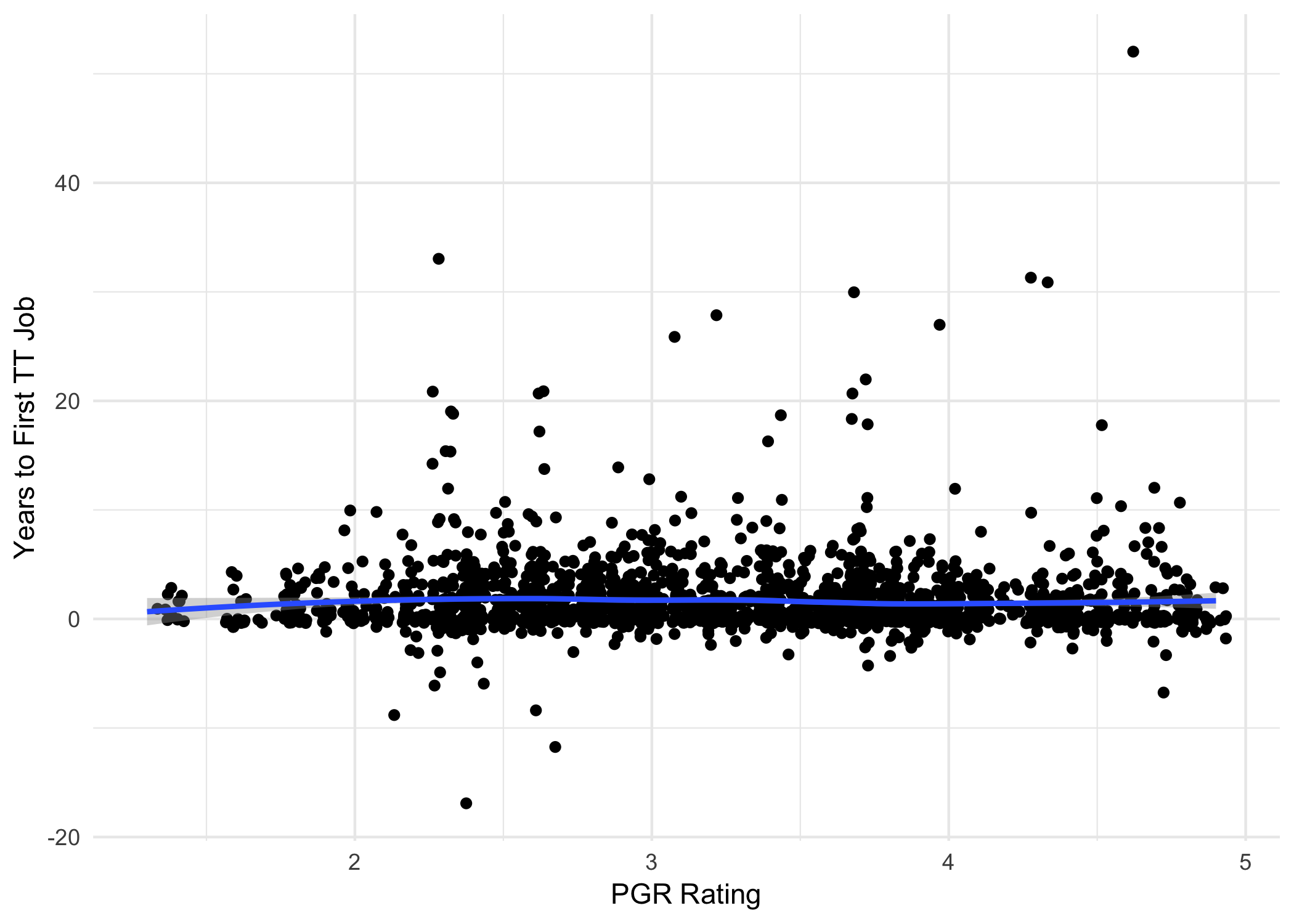
Wow, just… flat. Pretty much all the way across. And calculating the correlation, we get basically zero:
cor(df$mean, df$time_to_tt)
## [1] -0.03016805
There are some pretty weird anomalies though, like that outlier way out at the top right. Who took over 50 years to get their first TT job?!? Turns out that’s David C. Makinson, author of the classic 1965 paper, “The Paradox of the Preface”!
What on earth happened here? Makinson graduated from Oxford in 1965, and recently took up a visiting professorship at LSE in 2017, a difference of 52 years. That wasn’t his first tenured gig of course. But it’s the only one listed in the APDA database.
I guess any analysis of this size is bound to include at least a few such errors. (Shut up, I’m a dad.) But let’s try to minimize them.
As a first stab, we might just cut out any extreme outliers, say all
points where time_to_tt came out less than -2 or greater than 8.
df2 <- df %>% filter(-2 <= time_to_tt & time_to_tt <= 8)

ggplot(df2, aes(mean, time_to_tt)) +
 geom_jitter() +
 xlab("PGR Rating") + ylab("Years to First TT Job") +
 geom_smooth(method = "loess") +
 theme_minimal()
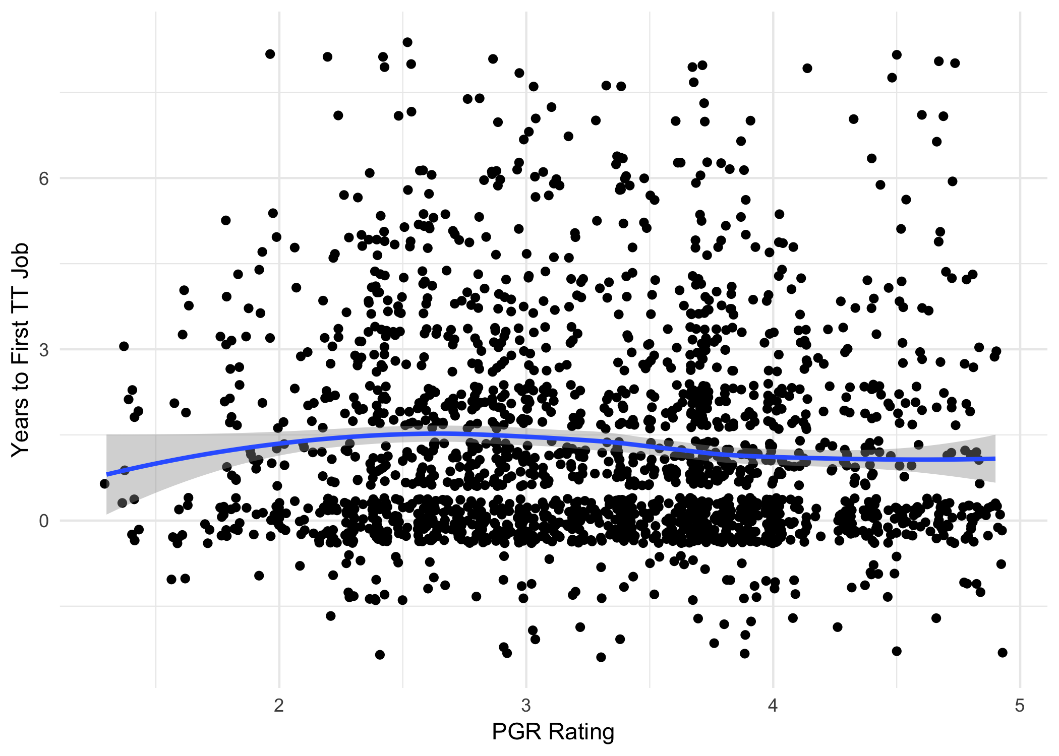
Things look a bit less flat now. Maybe there’s a slight dip in time-to-TT once PGR rating gets above 3 or so. But if so, it looks very small. And the overall correlation is again pretty much zero:
cor(df2$mean, df2$time_to_tt)
## [1] -0.06784644
Ok, one more try. Things work differently in different parts of the world. PhD programs and job markets differ in their practices between the US and the UK, between the UK and the rest of Europe, etc. So let’s try looking at just the US (the largest locale we have data for and the one I understand best):
df3 <- df2 %>% filter(locale == "US")

ggplot(df3, aes(mean, time_to_tt)) +
 geom_jitter() +
 xlab("PGR Rating") + ylab("Years to First TT Job") +
 geom_smooth(method = "loess") +
 theme_minimal()
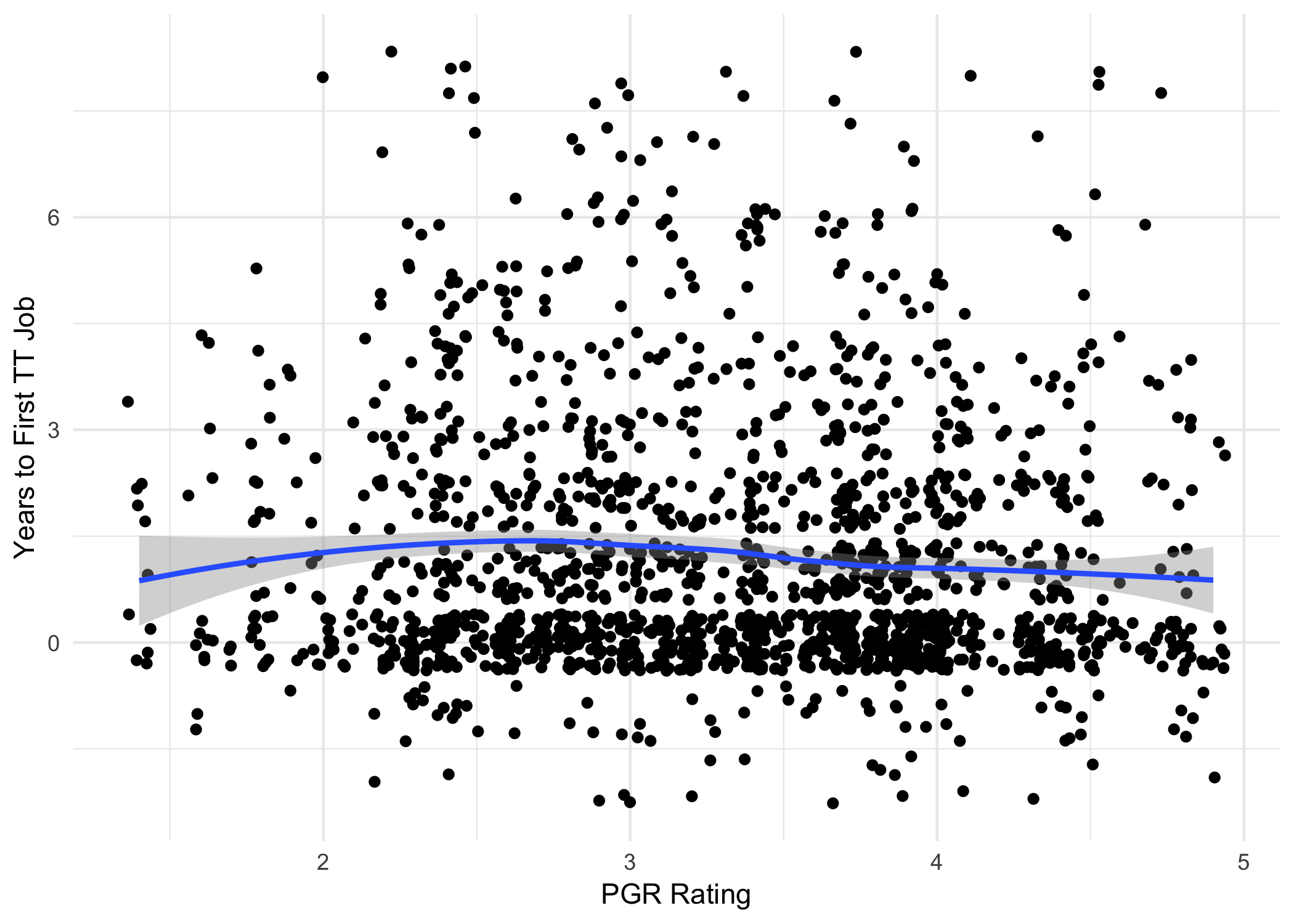
Again, it looks like there’s only a very slight dip as PGR rating exceeds 3, with a correlation very close to zero:
cor(df3$mean, df3$time_to_tt)
## [1] -0.06922355
Conclusion
We could go on slicing and dicing, and I don’t by any means see this as the last word. But my expectations have certainly been shaken up here. If there is a connection between prestige and time-to-TT, the available evidence suggests it’s much weaker than I would have guessed, and perhaps depends a lot on other factors.
Hopefully we’ll get a clearer picture of all this as the APDA database grows. Their focus so far has been on graduates from 2012–2016. So the earlier data is probably much less complete (see: Makinson). And not enough time has passed yet for the 2012–2016 data to be as informative about time-to-TT.
So even though this conclusion is striking, I still view it as tentative. #JustOneStudy