In our last two posts we established two key facts:

1. The set of possible probability assignments is convex.
2. Convex sets are “obtuse”. Given a point outside a convex set, there’s a point inside that forms a right-or-obtuse angle with any third point in the set.

Today we’re putting them together to get the central result of the accuracy framework, the Brier dominance theorem. We’ll show that a non-probabilistic credence assignment is always “Brier dominated” by some probabilistic one. That is, there is always a probabilistic assignment that is closer, in terms of Brier distance, to every possible truth-value assignment.

In fact we’ll show something a bit more general. We’ll show that there’s a probability assignment that’s closer to all the possible probability assignments. But truth-value assignments are probability assignments, just extreme ones. So the result we really want follows straight away as a special case.$ \renewcommand{\vec}[1]{\mathbf{#1}} \newcommand{\x}{\vec{x}} \newcommand{\y}{\vec{y}} \newcommand{\z}{\vec{z}} \newcommand{\v}{\vec{v}} \newcommand{\p}{\vec{p}} \newcommand{\q}{\vec{q}} \newcommand{\B}{B} \newcommand{\R}{\mathbb{R}} \newcommand{\EIpq}{EI_{\p}(\q)}\newcommand{\EIpp}{EI_{\p}(\p)} $

Recap

For reference, let’s collect our notation, terminology, and previous results, so that we have everything in one place.

We’re using $n$ for the number of possibilities under consideration. And we use bold letters like $\x$ and $\p$ to represent $n$-tuples of real numbers. So $\p = (p_1, \ldots, p_n)$ is a point in $n$-dimensional space: a member of $\R^n$.

We call $\p$ a probability assignment if its coordinates are (a) all nonnegative, and (b) they sum to $1$. And we write $P$ for the set of all probability assignments.

We call $\v$ a truth-value assignment if its coordinates are all zeros except for a single $1$. And we write $V$ for the set of all truth-value assignments.

A point $\y$ is a mixture of the points $\x_1, \ldots, \x_n$ if there are real numbers $\lambda_1, \ldots, \lambda_n$ such that:

• $\lambda_i \geq 0$ for all $i$,
• $\lambda_1 + \ldots + \lambda_n = 1$, and
• $\y = \lambda_1 \x_1 + \ldots + \lambda_n \x_n$.

We say that a set is convex if it is closed under mixing, i.e. any mixture of elements in the set is also in the set.

The difference between two points, $\x - \y$, is defined coordinate-wise: $$ \x - \y = (x_1 - y_1, \ldots, x_n - y_n). $$ The dot product of two points $\x$ and $\y$ is written $\x \cdot \y$, and is defined: $$ \x \cdot \y = x_1 y_1 + \ldots + x_n y_n. $$ As a reminder, the dot product returns a single, real number (not another $n$-dimensional point as one might expect). And the sign of the dot product reflects the angle between $\x$ and $\y$ when viewed as vectors/arrows. In particular, $\x \cdot \y \leq 0$ corresponds to a right-or-obtuse angle.

Finally, $\B(\x,\y)$ is the Brier distance between $\x$ and $\y$, which can be defined: $$ \begin{align} \B(\x,\y) &= (\x - \y)^2\\
&= (\x - \y) \cdot (\x - \y). \end{align} $$

Now let’s restate the two key theorems we’ll be relying on.

Theorem (Convexity).  The set of probability functions $P$ is convex.

We established this in Part 5 of this series. In particular, we showed that $P$ is the “convex hull” of $V$: the set of all mixtures of points in $V$.

Lemma (Obtusity).  If $S$ is convex, $\x \not \in S$, and $\y \in S$ minimizes $\B(\y,\x)$ as a function of $\y$ on the domain $S$, then for any $\z \in S$, $(\x - \y) \cdot (\z - \y) \leq 0$.

The intuitive idea behind this lemma, which we proved last time in Part 6, can be illustrated with a diagram: 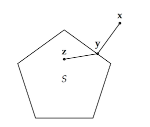Given a point outside a convex set, we can find a point inside (the closest point) that forms a right-or-obtuse angle with all other points in the set.

What we’ll show next is the natural and intuitive consequence: that point $\y$ is thus closer to any point $\z$ of $S$ than $\x$ is.

The Brier Dominance Theorem

Intuitively, we want to show that if the angle formed at point $\y$ with the points $\x$ and $\z$ is right-or-obtuse, then $\y$ must be closer to $\z$ than $\x$ is (in Brier distance).

Formally, a right-or-obtuse angle corresponds to a dot product less than or equal to zero: $(\x - \y) \cdot (\z - \y) \leq 0$. But if $\x = \y$, then the dot product will be zero trivially. So the precise statement of our theorem is:

Theorem.  If $(\x - \y) \cdot (\z - \y) \leq 0$ and $\x \neq \y$, then $\B(\x,\z) > \B(\y,\z)$.

Proof. To start, we establish a general identity via algebra: $$ \begin{align} \B(\x, \z) - \B(\x, \y) - \B(\y,\z) &= (\x - \z)^2 - (\x - \y)^2 - (\y - \z)^2\\
&= -2\y^2 - 2 \x \cdot \z + 2 \x \cdot \y + 2 \y \cdot \z\\
&= -2 (\x - \y) \cdot (\z - \y). \end{align} $$ Now suppose $ (\x - \y) \cdot (\z - \y) \leq 0$. Then, given the negative sign on the $-2$ in the established identity, $$ \B(\x, \z) - \B(\x, \y) - \B(\y,\z) \geq 0, $$ from which we derive $$ \B(\x, \z) \geq \B(\x, \y) + \B(\y,\z). $$ Now, since $\x \neq \y$ by hypothesis, $\B(\x,\y) > 0$. Thus $\B(\x,\z) > \B(\y,\z)$, as desired. $\Box$

It follows now that if $\x$ isn’t a probability assignment, there’s a probability assignment that’s closer to every truth-value assignment than $\x$ is.

Corollary (Brier Dominance). If $\x \not \in P$ then there is a $\p \in P$ such that $\B(\p,\v) < \B(\x, \v)$ for all $\v \in V$.

Proof. Fix $\x \not \in P$, and let $\p$ be the member of $P$ that minimizes $B(\y,\x)$ as a function of $\y$. The Convexity theorem tells us that $P$ is convex, so the Obtusity lemma implies $(\x - \p) \cdot (\v - \p) \leq 0$ for every $\v \in V$. And since $\x \neq \p$ (because $\x \not \in P$), the last theorem entails $\B(\p,\v) < \B(\x, \v)$, as desired. $\Box$

This is the core of the main result we’ve been working towards. Hooray! But, we still have one piece of unfinished business. For what if $\p$ is itself dominated??

Undominated Dominance

We’ve shown that credences which violate the probability axioms are always “accuracy dominated” by some assignment of credences that obeys those axioms. But what if those dominating, probabilistic credences are themselves dominated? What if they’re dominated by non-probabilistic credences??

For all we’ve said, that’s a real possibility. And if it actually obtains, then there’s nothing especially accuracy-conducive about the laws of probability. So we had better rule this possibility out. Luckily, that’s pretty easy to do.

In fact, the reals work here was already done back in Part 3 of the series. There we showed that Brier distance is a “proper” measure of inaccuracy: each probability assignment expects itself to do best with respect to accuracy, if inaccuracy is measured by Brier distance.

As a reminder, we wrote $\EIpq$ for the expected inaccuracy of probability assignment $\q$ according to assignment $\p$. When inaccuracy is measured in terms of Brier distance: $$ \EIpq = p_1 \B(\q,\v_1) + p_2 \B(\q,\v_2) + \ldots + p_n \B(\q,\v_n). $$ Here $\v_i$ is the truth-value assignment with a $1$ in the $i$-th coordinate, and $0$ everywhere else. What we showed in Part 3 was:

Theorem.  $\EIpq$ is uniquely minimized when $\q = \p$.

And notice, this would be impossible if there were some $\q$ such that $\B(\q,\v_i) \leq \B(\p,\v_i)$ for all $i$. For then the weighted average $\EIpq$ would have to be no larger than $\EIpp$. And this contradicts the theorem, which says that $\EIpq > \EIpp$ for all $\q \neq \p$.

So, at long last, we have the full result we want:

Corollary (Undominated Brier Dominance). If $\x \not \in P$ then there is a $\p \in P$ such that $\B(\p,\v) < \B(\x, \v)$ for all $\v \in V$. Moreover, there is no $\q \in P$ such that $\B(\q,\v) \leq \B(\p, \v)$ for all $\v \in V$.

So the laws of probability really are specially conducive to accuracy, as measured using Brier distance. Only probabilistic credence assignments are undominated.

Where to Next?

That’s a pretty sweet result. And it raises plenty of fun and interesting questions we could look at next. Here are three:

1. What about other ways of measuring inaccuracy besides Brier? Are there reasonable alternatives, and if so, do similar results apply to them?

2. What about other probabilistic principles, like Conditionalization, the Principal Principle, or the Principle of Indifference? Can we take this approach beyond the probability axioms?

3. Speaking of the probability axioms, we’ve been working with a pretty paired down conception of a “probability assignment”. Usually we assign probabilities not just to atomic possibilities, but to disjunctions/sets of possibilities: e.g. “the prize is behind either door #1 or door #2”. Can we extend this result to such “super-atomic” probability assignments?

We’ll tackle some or all of these questions in future posts. But I haven’t yet decided which ones or in what order.

So for now let’s just stop and appreciate the work we’ve already done. Because not only have we proved one of the most central and interesting results of the accuracy framework. But also, in a lot of ways the hardest work is already behind us. If you’ve come this far, I think you deserve a nice pat on the back.