Last time we saw that Euclidean distance is an “unstable” way of measuring inaccuracy. Given one assignment of probabilities, you’ll expect some other assignment to be more accurate (unless the first assignment is either perfectly certain or perfectly uncertain).

That’s why accuraticians don’t use good ol’ Euclidean distance.

Instead they use… well, there are lots of alternatives. But the closest thing to a standard one is Brier distance: the square of Euclidean distance.

Here’s Euclid’s formula for the distance between two points $(a, b)$ and $(c, d)$ in the plane: $$ \sqrt{ (a - c)^2 + (b - d)^2 }. $$ And here’s Brier’s: $$ (a - c)^2 + (b - d)^2. $$ So, to get from Euclid to Brier, you just take away the square root.

That makes a world of difference, it turns out. Brier distance isn’t unstable the way Euclidean distance is. But we’ll see that it’s enough like Euclidean distance to vindicate the argument for the laws of probability we began with last time.

But first, a fun fact.

Fun Fact

Brier distance comes from the world of weather forecasting. Glenn W. Brier worked for the U. S. Weather Bureau, and in a 1950 paper he proposed his formula as a way of measuring how well a weather forecaster is doing at predicting the weather.

Suppose you say there’s a 70% chance of rain. If it does rain, you’re hardly wrong, but you’re not exactly right either. Brier suggested assessing a forecaster’s probabilities by taking the square of the difference from $1$ when it rains, and from $0$ when it doesn’t.

Well, actually, he proposed taking the average of those squares. But we’ll follow the recent philosophical literature and keep it simple: we’ll just use the sum of squares rather than its average.

Now on to the substance. Two facts about Brier distance make it useful as a replacement for Euclidean distance.

Euclid and Brier are Ordinally Equivalent

First, Brier distance is ordinally equivalent to Euclidean distance. Meaning: whenever a distance is larger according to Euclid, it’s larger according to Brier too. And vice versa.

How do we know that? Because Brier is just Euclid squared, and squaring a larger number always results in a larger number (for positive numbers like distances, anyway). If $D$ is the distance from Toronto to the sun, and $d$ is the distance from Toronto to the moon, then $D^2 > d^2$. It’s further to the sun than to the moon, both in terms of Brier distance and Euclidean distance.

So, when we’re comparing distances from the truth, Brier distance behaves a lot like Euclidean distance. In particular, what we learned from our opening diagram about Euclidean distance holds for Brier distance, too.

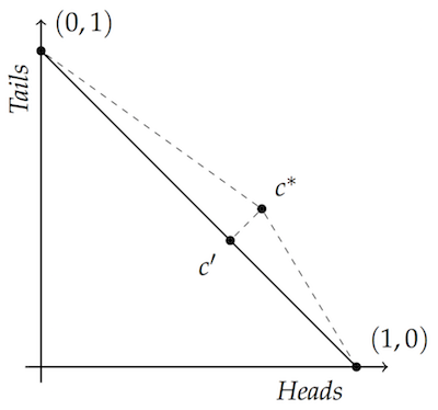
Not only is $c’$ closer to both vertices than $c^*$ in Euclidean terms, it’s also closer in terms of Brier distance.

Brier is Stable

Second, Brier distance doesn’t lead to the kind of instability that made Euclidean distance problematic. To see why, let’s rerun our expected inaccuracy calculations from last time, but using Brier distance instead of Euclid.

Suppose your credences in Heads and Tails are $p$ and $1-p$. What’s the expected inaccuracy of having some credence $q$ in Heads, and $1-q$ in Tails?

Well, the Brier distance between $(q, 1-q)$ and $(1,0)$ is: $$(q - 1)^2 + ((1-q) - 0)^2.$$ And the Brier distance between $(q, 1-q)$ and $(0,1)$ is: $$(q - 0)^2 + ((1-q) - 1)^2.$$ We don’t know which of $(1,0)$ or $(0,1)$ is the “true” one. But we have assigned them the probabilities $p$ and $1-p$, respectively. So we can calculate the expected inaccuracy of $(q, 1-q)$, written $EI(q, 1-q)$: $$ \begin{align} EI(q, 1-q) &= p \left( (q - 1)^2 + ((1-q) - 0)^2 \right)\\
&\quad + (1-p) \left( (q - 0)^2 + ((1-q) - 1)^2 \right)\\
&= 2 p (1 - q)^2 + 2(1-p) q^2\\
&= 2 p q^2 - 4pq + 2p + 2q^2 - 2pq^2\\
&= 2q^2 - 4pq + 2p \end{align} $$ Now that last line might look like a mess. But it’s really just a quadratic equation, where the variable is $q$. Remember: we’re treating $p$ as a constant since that’s the credence you hold. And we’re looking at potential values of $q$ to see which ones minimize the quantity $EI(q, 1-q)$, given a fixed credence of $p$ in heads.

So which value of $q$ minimizes this quadratic formula? You might remember from algebra class that a quadratic equation of the form: $$ ax^2 + bx + c $$ is a parabola, with the bottom of the bowl located at $x = -b/2a$. (Or, if you know some calculus, you can take the derivative and set it equal to $0$. Since the derivative here is $2ax + b$, setting it equal to $0$ yields, again, $x = -b/2a$.)

In the case of our formula, we have $a = 2$ and $b = -4p$. So the minimum happens when $q = 4p/4 = p$. In other words, given credence $p$ in heads, expected inaccuracy is minimized by sticking with that same credence, i.e. assigning $q = p$.

So, to complement our result about Euclidean distance from last time, we have a

Theorem.  Suppose $p \in [0,1]$. Then, according to the probability assignment $(p, 1-p)$, the expected Brier distance of any alternative assignment $(q, 1-q)$ from the points $(1,0)$ and $(0,1)$ is uniquely minimized when $p = q$.

Proof.  Scroll up! $\Box$

Proper Scoring Rules

When a measure of inaccuracy is stable like this, it’s called proper (or sometimes: immodest).

There are lots of other proper ways of measuring inaccuracy besides Brier. But Brier tends to be the default among philosophers writing in the accuracy framework, at least as a working example. Why?

My impression (though I’m no guru) is that it’s the default because:

1. Brier is a lot like Euclidean distance, as we saw. So it’s easier and more intuitive to work with than some of the alternatives.
2. Brier tends to be representative of other proper/immodest rules. If you discover something philosophically interesting using Brier, there’s a good chance it holds for many other proper scoring rules.
3. Brier has other nice mathematical properties which, according to authors like Richard Pettigrew, make it The One True Measure of Inaccuracy. (It may have some odd features too, though: see this post by Brian Knab and Miriam Schoenfield, for example.)

How does our starting argument for the laws of total probability fare if we use other proper scoring rules, besides Brier? Really well, it turns out!

The key fact our diagram illustrates doesn’t just hold for Euclidean distance and Brier distance. Speaking very loosely: it holds on any proper way of measuring distance (but do see sections 8 and 9 of Joyce’s 2009 for the details before getting carried away with this generalization; or see Theorem 4.3.5 of Pettigrew 2016).

Proving that requires grinding through a good deal of math, though. So in these posts we’re going to stick with Brier distance, at least for a while.

Begging the Question?

We started these posts with an illustration of an influential argument for the laws of probability. But we quickly switched to assuming those very same laws in the arguments that followed.

For example, to illustrate the instability of Euclidean distance, I chose a point on the diagonal of our diagram, $(.6, .4)$. And in the theorem that generalized that example, I assumed probabilistic assignments like $(p, 1-p)$ and $(q, 1-q)$, which add up to $1$.

So didn’t we beg the question when we motivated switching from Euclid to Brier?

To some extent: yes. We are assuming that reasonable ways of measuring inaccuracy can’t be so hostile to the laws of probability that they make almost all probability assignments unstable.

But also: no. We aren’t assuming that the laws of probability are absolute and inviolable, just that they’re reasonable sometimes. Euclidean distance would rule out probabilistic credences on pretty much all occasions. So it conflicts with the very modest thought that following the laws of probability is occasionally reasonable. So, even if you’re just a little bit open to the idea of probability theory, Euclidean distance will seem pretty unfriendly.¹

Perhaps most importantly, though: the motivation I’ve given you here for moving from Euclid to Brier isn’t the official one you’ll find in an actual, bottom-up argument for probability theory, like Richard Pettigrew’s. His argument starts from a much more abstract place. He starts with axioms that any measure of inaccuracy must obey, and then narrows things down to Brier.

So there’s the official story and the unofficial story. This post gives you the unofficial story, to help you get started. Because the official story is often really hard to understand. Not only is the math way more abstract, but the philosophical motivations are often hard to suss out. Because—and this is just between you and me now—the people telling the official story actually started out with the unofficial story, and then worked backwards until they came up with an officially respectable story that doesn’t beg the question quite so obviously.

Ok, that’s unfair. Here’s a more even-handed (and better-informed) way of putting it, from Kenny Easwaran’s review of Pettigrew’s book:

Some philosophers have a vision of what they do as starting from unassailable premises, and giving an ironclad argument for a conclusion. However, I think we’ve all often seen cases where these arguments are weaker than they seem to the author, and with the benefit of a bit of distance, one can often recognize how the premises were in fact motivated by an attempt to justify the conclusion, which was chosen in advance. Pettigrew avoids the charade of pretending to have come up with the premises independently of recognizing that they lead to the conclusions of his arguments. Instead, he is open about having chosen target conclusions in advance […] and investigated what collection of potentially plausible principles about accuracy and epistemic decision theory will lead to those conclusions.